A key geographical question throughout the human experience has been: “Where am I?”. In classical Greece and China, attempts were made to create logical grid systems of the world to answer this question. The ancient Greekgeographer Ptolmey created a grid system and listed the coordinates for places throughout the known world in his book Geography. But it was not until the middle ages that the latitude and longitude system was developed and implemented. This system is written in degrees (°).
When looking at a map, latitude lines run horizontally. They are also known as parallels since they are parallel and are at equal distant from each other. Each degree of latitude is approximately 111 km apart. Degrees latitude are numbered from 0° to 90°. Latitude 0° corresponds to the Equator, the imaginary line which divides our planet into the Northern and Southern hemispheres. Latitudes 90° and -90° refer to the North Pole and the South Pole respectively.
The vertical longitude lines are also known as meridians. They converge at the poles and are widest at the Equator. Longitude 0° is located at Greenwich, England. The degrees continue 180° (or 180° east) and -180° (or 180° west) where they meet and form the International Date Line in the Pacific Ocean. Greenwich, the site of the British Royal Greenwich Observatory, was established as the site of the Prime Meridian by an international conference in 1884.
There are two methods of expressing fractions of degrees. The first method divides each degree into 60 minutes (1° = 60’), then each minute into 60 seconds (1’= 60”). This system is called DMS (degrees, minutes, seconds). The symbol for degrees is °, for minutes is ‘, and for seconds is “. For example Rome, Italy is located at the latitude 41° 53’00”, longitude 12° 30’00”. The second method states the fraction as a decimal of a degree. This is the DD (decimal degree) system. With this system the position of Rome is: latitude 41.88333°, longitude 12.5°.
To convert from the DMS system to decimal degrees (DD) you can use a simple formula: (degrees)+(minutes/60)+(seconds/3600) = decimal degrees.
The conversion from DD to DMS is a little more complicated, and will be explained with the following example. Suppose you have the decimal degree reading of 5.23456°. To convert it to the DMS system, you first subtract the whole degree. 5° is the whole degree, so 5.23456°-5°=0.23456°. Then you multiply the remaining fraction with 60 minutes (0.23456° * 60’=14.0736’), 14’ is the whole minutes. After this you multiply the fraction of the minutes with 60 seconds (14.0736’-14’=0.0736’, 0.0736’*60”=4.416”), 4.416” are the remaining seconds. The DMS version of 5.23456° is 5° 14’ 4.416”
1. Open ArcView, a new Project, and a new View. Add from the folder ‘09_Degrees’ the Themes ‘Pais_pesca_fishing_villages.shp’ and ‘district.shp’ to the View.
2. Change the background colour (menu bar: View/Properties.../Select color) to blue. Zoom in on the southeastern part of the View, until you have almost the same view as in Figure 11.1. Autolabel the villages Theme with ‘Name’.
FIGURE 11.1
Marine fishing villages
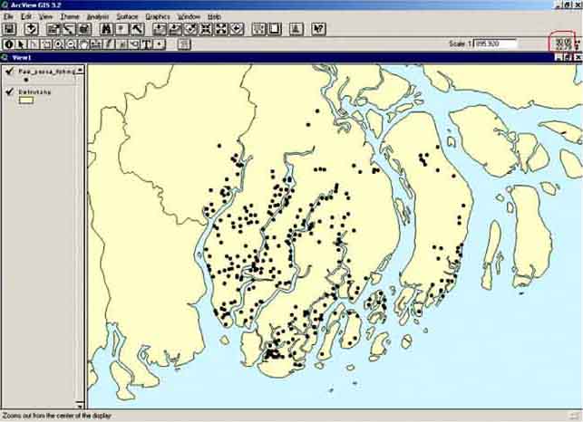
When you move the pointer over the View, you will see that in the upper right corner some numbers are changing. These numbers indicate the location on the map in decimal degrees. With these numbers every point in the View is georeferenced: they represent an exact location somewhere on the surface of the Earth. If you look at the map, and move the pointer over the villages named Lais and Cambarellus, you will see that in the upper right hand corner the values are: (for Lais) X:90.49 and Y:22.16, and (for Cambarellus) X:90.69 and Y:22.04. In the attributes table of the villages theme these decimal degrees are even more precise:
TABLE 11.1
Location of villages in decimal
degrees
|
|
X_coord |
Y_coord |
DMS Longitude |
DMS Latitude |
|
Lais |
90.48827 |
22.15964 |
|
|
|
Cambarellus |
90.68600 |
22.03698 |
|
|
Can you calculate in Excel or on a calculator from the above decimal degrees the DMS longitude and latitude values of both villages?
The other way around is also possible. Suppose you have collected data in a village, and you want to put them in your GIS database. You know the latitude-longitude position (in the DMS system), because you have read that from a map, or from a GPS (Global Positioning System) reader. How do you convert these values to decimal degrees, so that you can use them in a GIS. Calculate the decimal degrees of the following position in the DMS system:
TABLE 11.2
Decimal degree conversion to DMS
exercise
|
|
Latitude |
Longitude |
|
DMS |
22° 10’1.38” |
90° 8’32.352” |
|
Decimal Degrees |
|
|
Find the village that belongs to this position in the View by moving the pointer (it is best to use the Identify pointer, and Zoom in or out when needed), and looking at the numbers in the upper right hand corner. What is the name of this village? (it should be Astacus). Close the project and Exit ArcView.
In 2000 the Department of Fisheries carried out a survey in the coastal district of Pais Pesca. The objective was to locate the villages where marine fishers were living and to collect socio-economic data. You can find these data in the Excel file: ‘Marine frame survey exercise.xls’ in the ‘09_Degrees’ folder. Open this file (in Excel of course!) (Figure 11.2).
FIGURE 11.2
Excel file with data of the survey of the
coastal district
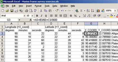
You can see that the file contains GPS readings with degrees, minutes, and seconds in separate cells. Following these are two columns where decimal degrees are supposed to come, filled with question marks. These two columns are followed by columns with data concerning the villages. First you have to convert the GPS readings (in the DMS system) into decimal degrees (DD).
1. Convert the GPS readings into Decimal degrees on the Excel sheet. (Remember the formula?: (degrees)+(minutes/60)+(seconds/3600) = decimal degrees, see Figure 11.3).
FIGURE 11.3
Excel sheet with converted GPS readings (DMS to DD)
2. Now the sheet is almost ready to be used in ArcView. ArcView unfortunately does not use Excel files, but does use ‘.dbf’ files, so you have to convert the sheet that you have created into a.dbf file. Go via the Excel menu bar to: File/Save As.... The Save As screen pops up, where you change the file into a ‘.dbf’ file (Figure 11.4). Make sure that before you save this file as a ‘.dbf’ file, the format of the cells containing the decimal degrees (X_COORD and Y_COORD) is: Number with at least six decimals (select the cells, then via menu bar: Format/Cells..., etc.).
FIGURE 11.4
Excel sheet converted to.dbf file
3. When you save the sheet as a ‘.dbf’ file, you will get the message starting with: ‘The selected file type does not support workbooks that contain multiple sheets’. Because you are only interested in the active sheet click OK. You have now exported the Excel file in a format that you can use in ArcView. You will now be able to import the data and use them into the View you have of Pais Pesca. For more information on working with Microsoft Excel and ArcView, have a look at Annex B: ArcView and Microsoft Excel on page 150.
4. Open ArcView, Open a New Project, Open a New View, and add the Theme ‘district.shp’ to the View. Close the View, go to Tables and press Add. Look for the file you just have created (‘Marine frame survey exercise.dbf’) and press OK (Figure 11.5).
FIGURE 11.5
Importing the ‘Marine frame survey exercise.dbf’ file
5. Open the table and make sure the data are still correct. Pay special attention that in the field X_COORD and Y_COORD you have values with six decimals. If this is not the case, you have to do the conversion from Excel sheet to ‘.dbf’ file again, but now pay attention that the cells containing the decimal degrees (X_COORD and Y_COORD) have a number format, with 6 decimals. Maybe you also have to Copy the cells and Paste special (value) them.
6. If the data look okay, close the table and go to Views. Open the View. Now you want to add the data to this View (where the district theme is already present). Go via the menu bar to: View/Add Event Theme... (Figure 11.6).
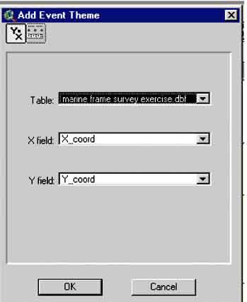
7. The Add Event window will pop up. Here you have to insert which file you want to add (‘Marine frame survey exercise. dbf’), and which fields contain the X and Y coordinates (X_COORD and Y_COORD) (Figure 11.7).
FIGURE 11.6
Adding a theme with collected data from
the marine frame survey
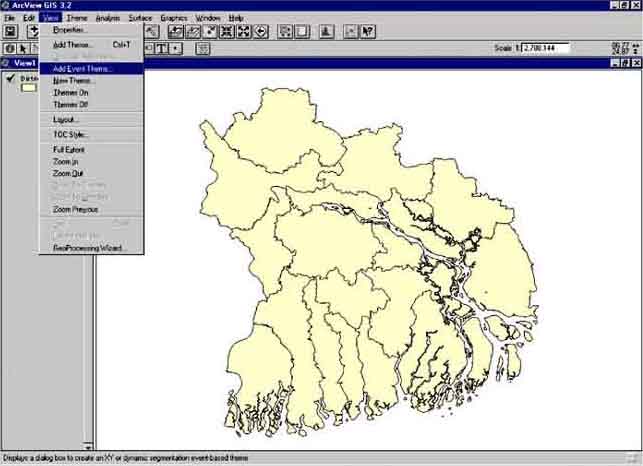
FIGURE 11.7
The Add Event Theme window
1. Once you are sure the correct file will be used, and the correct field will be used for the X and Y coordinates press OK. You will see a new Theme appear in the View, called ‘Marine frame survey exercise.dbf’. Check the View Box and you will see that points appear in the southeast corner of Pais Pesca.
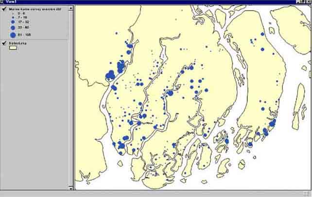
2. You can now analyse the data collected by the Department of Fisheries. Make a View showing the villages and the number of boats with graduated symbol in the Legend Editor (Figure 11.8).
FIGURE 11.8
The villages with the number of
boats
Also the distribution of the number of gear, and the type of gear is possible to show. Make this view (Figure 11.9).
FIGURE 11.9
The distribution of gear
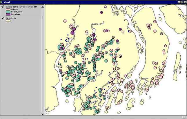
This last exercise needed you to calculate the total number of gear, by adding a field and calculating the total number of gear. If you have forgotten how to do this, have a look at: Adding a field and making calculations in a table, on page 31.
In the previous chapters and exercises you have seen how to display data joined to a point Theme in the form of histograms or graduated colours and graduated symbols. The best plot is the graduated symbol as it gives in one view the distribution of the fishing boats along the coast and allows to identify quickly where the villages with large numbers of boats are.
The different forms of displaying data in GIS discussed until now are not appropriate if you want to know why there is a large number of boats, or large numbers of Tilapia in a certain area, or want to know if there is a gradient in the abundance of fish stocks and to which factors this gradient is related. For this you have to interpolate between the data at different locations, which is often done with a contour plot that connects data points with the same values.