Installing Kriging Scripts
Kriging interpolation of data is a regular part of the Spatial Analyst software, however, to use this you need to be able to program in Avenue, the programming language of ArcView. Fortunately there are several free scripts for Kriging available on the Internet. An example of such a tool is the Spatial Tools ArcView extension that can be downloaded from (among others): http://www.absc.usgs.gov/glba/gistools/. You can find the file and its documentation in the folder /extensions/kriging on the CD. In order to be able to use this add-in you have to:
1. Copy the ‘g2i.dll’ file from the ‘/extensions/kriging’ on the CD to the ArcView Bin32 folder (the path will look like the following, although the drive letter may not be the same, and also you might be using a different version of ArcView): C:\ESRI\AV_GIS30\ARCVIEW\BIN32.
2. Copy the ‘Spatiatools.avx’ file to the ArcView Ext32 directory (The same comment as made above applies here): C:\ESRI\AV_GIS30\ARCVIEW\EXT32.
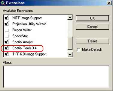
After you have opened ArcView, Go to File/Extensions... via the menu bar and select Spatial Tools 3.4 (Spatial Analyst needs to be selected first) (Figure C.1).
FIGURE C.1
Making the Spatial Tools extension active
in ArcView
What is Kriging[49]
Kriging is a powerfull statistical interpolation method. The technique was co-developed by Georges Matheron (a French geomathematician) and D.G. Krige (a South African mining engineer) to analyse geochemical data to find gold deposites (and it worked!). The difference between ordinary interpolation in ArcView and Kriging is that with Kriging an initial structural spatial analysis is carried out, looking at the variance and autocorrelation of the data. The results of the analysis are then used to select the interpolation model and carry out the interpolation. Kriging is an estimation method that is associated with the acronym BLUE (Best Linear Unbiased Estimator). It is linear since the estimated values are weighted linear combinations of available data. It is unbiased because the mean of the error is zero. It is best since it aims at minimizing the variance of the errors. Therefore the word Kriging is synonymous with optimal prediction.
In Kriging a semivariogram is constructed which expresses the spatial variation in the data. Then the mathematical model of the semivariogram is used in calculating estimates of the surface at the different locations. Kriging will result in two images, a surface of estimates and a surface of estimated variances. The latter image can be used to identify problems with the fit of the model to the sample data by revealing relative differences in the model fit across the study area. For a more detailed explanation you can visit: http://www.nbb.cornell.edu/neurobio/land/OldStudentProjects/cs490-94to95/clang/kriging.html.
Semivariogram
Semi variance is a measure of the degree of spatial dependence between samples. The magnitude of the semi variance between points depends on the distance between the points. A smaller distance yields a smaller semi variance and a larger distance results in a larger semi variance. Given two locations x and (x+h), a measure of one half of the mean square difference (the semivariance) produced by assigning the values z(x+h) to the value z(x), where h (known as the lag) is the inter-sample distance. Plotting the semivariance versus the lag h gives a semivariogram. Mathematically the semivariance is written as:

where:
|
y*(h) |
is the calculated value of the variogramme or covariance at a distance h. |
|
Z |
is the attribute value. |
|
N |
is the number of pairs of sample points separated by h. |
The summation is carried out over all distances h.
The plot of the semi variance as a function of distance from a point is referred to as a semi variogramme (Figure C.2). The semi variance increases as the distance increases until it reaches a maximum at a certain distant away from a point. Then the semi variance will equal the variance around the average value, and will therefore no longer increase, causing a flat region to occur on the semi variogram, which is called the sill.
FIGURE C.2
A semi variogramme
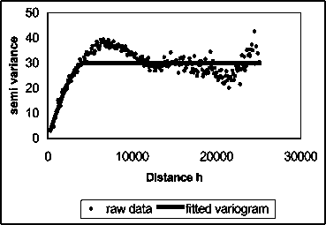
From the point of interest to the distance where the flat region begins is termed the range of the regionalized variable. Within this range, locations are spatially autocorrelated to each other, and all known samples contained in this region, also referred to as the neighbourhood, must be considered when estimating the unknown point of interest. The centre of the neighbourhood is usually the unknown value. In order to determine this, unknown, value, all known values within the neighbourhood are assigned weights using the semivariogram. These weight and known values are then used to calculate the unknown value. The kriged estimates are the best linear unbiased estimates of the surface at the specified locations, provided the surface is stationary and the correct form of the semivariogram has been determined. The Kriging script we use provides two grids:
The data grid; and
A grid providing the variance.
A large advantage of Kriging is that with the made variance grid of the interpolation you can evaluate how accurate the estimated values are and provide you with evidence of problems of the fit.
Kriging with Spatial Tools
Spatial tools 3.4 provides two Kriging options:
Ordinary Kriging; this is the most commonly used and the simplest form of Kriging. It assumes that local means are not necessarily closely related to the population mean, and which therefore uses only the samples in the local neighbourhood for the estimate.
Universal Kriging, also known as Kriging with a trend. It is used when a trend or slow change of the average values in the samples exists.
Further, there are five mathematical forms the semivariogram can be made:
Spherical: this calculated the variogramme as a modified quadratic function for which at some distance Ao, pairs of points will no longer be auto correlated and the variogramme reaches an asymptote.
Circular: uses a circular neighbourhood search model with a certain radius.
Exponential: the exponential model is similar to the spherical in that it approaches the sill gradually. However, different from the spherical in the rate the sill is approached and in the fact that the model and the sill never actually converge.
Gaussian: the gaussian or hyperbolic model is similar to the exponential but it assumes a gradual rise for the y-intercept.
Linear with sill: this model is similar to the linear model except that at some distance pairs of points will be no longer auto correlated and the variogram will reach an abrupt asymptote.
An example of Kriging with data from Pais Pesca
Try to apply Kriging on different data of Lake Kadim in Pais Pesca.
1. Start ArcView, Open a New Project, New View. Add the following Themes from the ‘AN_Kriging’ folder: ‘Lake Kadim.shp’, ‘Lake Kadim data.shp’, and ‘Pais_pesca_country.shp’.
2. Check the projection and the working directory. Go to File/Extensions... and make ‘Spatial tools 3.4’ active. Activate the ‘Lake Kadim data.shp’ Theme, and zoom with the ‘Zoom to Active Theme(s)’button in the button bar.
3. Now you can start Kriging data of Lake Kadim. First waterdepth data will be kriged.
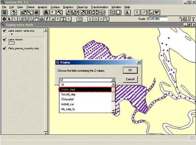
4. Activate the ‘Lake Kadim data.shp’ Theme. Go to Analysis/Kriging Interpolation... in the menu bar. The Kriging window will pop up and from the drop down list you select ‘water_dept’ as the field in the table you want to Krig (Figure C.3). Click OK.
FIGURE C.3
Selecting the Z-value for
Kriging
5. You will be asked if you want to use a barrier to limit the extent of the interpolation. Click No, as you have no line barrier (Figure C.4).
FIGURE C.4
Use barrier?
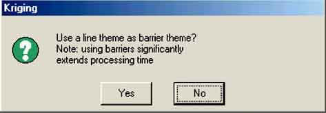
FIGURE C.5
Selecting the type of Kriging

6. A new window pops up where you have to select the type of Kriging. You do not suspect that there is a trend in the water depth data so you select ‘Ordinary Kriging’(Figure C.5) and click OK.
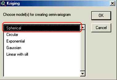
7. A window will pop up where you have to select what type of model you want to use for the semivariogram. Select ‘Spherical’(Figure C.6) and click OK.
FIGURE C.6
Selecting the type of model to use for
Kriging
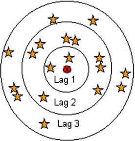
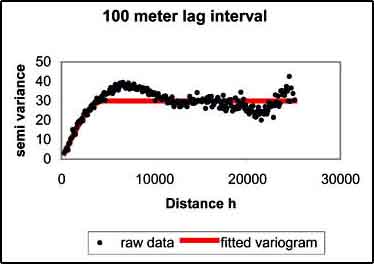
8. The Lag interval window will pop up. In here you enter the lag interval to calculate the semivariance of the dataset (Figure C.7). This parameter strongly influences the form of the variogram. Further it is impractical to plot a variance for each scatter point with respect of the other scatter points. Therefore the distances are subdivided into a number of intervals called lags (Figure C.8). The distance between each pair of scatter points is checked to see which lag interval it lies in. The variance for all pairs of points whose separation distance falls within the same lag interval is averaged. The resulting average is plotted in the semivariogram versus the distance corresponding to the lag interval. Therefore, there is one point in the variogram for each lag. A small lag interval results in a large number of points in your variogramme, but here each point is the average of a limited number of scatter points. Increasing the lag interval will reduce the number of points in your variogram, but each average is made up of an increasing number of scatter points increasing the accuracy (Figures C.20 and C.21). There are some rules selecting the right number of intervals (Journel and Hubregts, 1978), but you can also get a reasonable guess by looking at the resulting semivariogram. It is a compromise between the accuracy of the calculated semivariance and a sufficient number of data points in the semivariogram to allow reasonable fitting of the curve.
FIGURE C.7
The Lag Interval window

FIGURE C.8
The lag scheme
9. Enter 100 metres as lag interval and click OK.
10. The semivariance will be calculated (This may take some time!). After a while a window will appear, saying: ‘Write all variogram data to a file? Note: the file svgram1.svg that is added to the project is overwrtitten each time this script is run’, indicating that the calculations are made. Click on Yes.
11. In the next window you will be asked to indicate the file-type you want to save the data in. Select dBASE and click OK (Figure C.9).
FIGURE C.9
Saving the result of the kriging as a dBASE file
FIGURE C.10
Naming the variogram
12. In the next window provide the name you want to give to the data table (Figure C.10).
13. The next window which pops up (Figure C.11) gives the different codes which are used in the saved table, click OK.
FIGURE C.11
Coding of the variogram
FIGURE C.12
Layout of the generated variogram
14. The created semivariogram appears (Figure C.12). Click OK. You will be asked if you want to print out the semivariogram. Make your choice and click the according button.
15. Now you will be asked to start the interpolation (Figure C.13). click Yes and select ‘Spherical’ in the next window (Figure C.14).
FIGURE C.13
Start interpolation?
FIGURE C.14
Chosing the method of interpolation
16. An explanation for the next step will appear, read the explanation and click OK.
17. In the next window select ‘Fixed’ from the dropdown box (Figure C.15).
FIGURE C.15
Chosing the type of radius
FIGURE C.16
Entering the radius parameters
18. The Output Gird Specification window pops up. Select Same as Display in the Output Grid Extent box, and 100 m for the Output Gird Cell Size.
19. and keep the radius at 1 000 (Figure C.16).
20. The last question is ‘Create output variance grid?’(Figure C.17). Click Yes.
FIGURE C.17
Creating an output grid?
21. The interpolation will start and both grids will be added to the View. Reclassify the legend and you will have the grids as presented in Figure C.18 and Figure C.19
FIGURE C.18
Kriged waterdepth
FIGURE C.19
Variance of water depth after Kriging
Try now to Krig yourself the other data of the Theme ‘Lake Kadim data.shp’ (distribution of: adult carp, carp larvae, Secchi depth, watertemp, and clupeid larvae, and concentration of chlorophyll).
FIGURE C.20
Semi variogram made with a 5 metres lag
interval
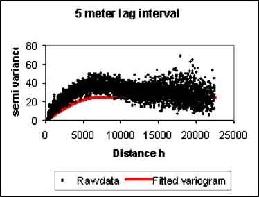
FIGURE C.21
Semi variogrammade with a 100 metres lag
interval
This annex is merely an introduction to Kriging. Kriging is a complex procedure that requires greater knowledge about spatial statistics than can be covered in this annex. Before applying Kriging, you should acquire a thorough understanding of the fundamentals of Kriging and have assessed the appropriateness of your data for modelling with this technique. If you would like to learn more about Kriging, some excellent references about Kriging and statistical interpolation are listed below:
Burrough, P.A. 1986. Principles of Geographic Information Systems for Land Assessment., Oxford University Press, New York.
Heine, G.W. 1986. A controlled study of some two-dimensional interpolation method. COGS Computer Contributions, 3(2): 60-72.
McBratney, A.B. & Webster R., 1986. Choosing functions for semi-variograms of soil properties and fitting them to sampling estimates. Journal of Soil Science, 37: 617-639.
Oliver, M.A. 1990. Kriging: a method of interpolation for geographical information systems. International Journal of Geographic Information Systems, 4 (4): 313-332.
Press, W.H., Teukolsky, S.A., Vetterling, W.T. & Flannery, B.P. 1988. Numerical Recipes in C: The Art of Scientific computing. New York, Cambridge University Press. 904 pp.
Royle, A.G., Clausen F.L. & Frederiksen P., 1981. Practical universal Kriging and automatic contouring. Geoprocessing, 1: 377-394.
|
[49] Adapted from: |