Science builds models or theories to explain phenomena. One observes phenomena and then looks for relations, causes and effects. Observations are made about the evolution of a magnitude (characteristics) with time (or with other characteristics) and possible causes (factors) are explored. Examples:
2.1.1 STRUCTURE OF A MODEL
Basic assumptions
The assumptions to serve as a basis for a model should:
Usually basic assumptions are related to the evolution of the characteristics. So, they are established on the variation rate of those characteristics and they do not need to be proved.
Relations (properties)
"results" or "conclusions" of the model.
Verification
This implies the application of statistical methods and sampling techniques to check the agreement of the results with the observations.
Improvement
Advantages
2.1.2 SOME TYPES OF MODELS USED IN STOCK ASSESSMENT
Production Models
The production models are also designated as General Production models, Global models, Synthetical models or Lotka-Volterra type models. These models consider the stock globally, in particular the total abundance (in weight or in number) and study its evolution, the relation with the fishing effort, etc.. They do not consider the structure of the stock by age or by size.
Structural Models
These models consider the structure of the stock by age and the evolution of the structure with time. They mainly recognize that the stock is composed of individuals of different cohorts, and, consequently, of different ages and sizes. So, they analyse and they project the stock and the catches for the coming years, by following the evolution of its different cohorts.
This manual will not follow the chronological construction of the models. It was thought to be more convenient to deal firstly with the structural models and afterwards with the production models.
The basic assumptions of a model, for the evolution of a characteristic, require the concept of variation rate of the characteristic related to time (or to other characteristics).
Figure 2.1 Evolution of the length (L) of an individual with time (or age) (t)

In order to generalize the study of the rates, the characteristic L in the example above will be substituted by y, and the associated variable will not be time, t, but the variable x. To study the stock assessment models and to make this study easier, it will be considered that the function y will only assume real and positive values.
2.2.1 ABSOLUTE MEAN RATE - amr (y)
Consider y a function of x and the interval i with the limits (xi, xi+1)
Figure 2.2 Function y= f(x) with variation in the interval i

Let:
Δxi = xi+1 - xi be the size of the interval
yi = the value of y when x = xI
yi+1 = the value of y when x = xi+1
The variation of y in the interval Δxi will be Δyi = yi+1 - yi
The absolute mean rate, amr (y), of the variation of y within the interval Δxi, will be:

Graphically:
Figure 2.3 Absolute mean rate of the variation of y within the interval Δxi

Slope of the secant =
 = amr (y) during
Δxi
Note: amr (y) is known in physics as the mean velocity of the variation of y with x, in the interval Δxi.
2.2.2 ABSOLUTE INSTANTANEOUS RATE - air (y)
Let y be a function of x
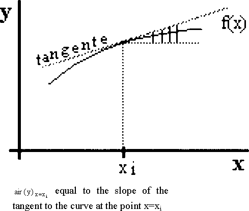
The absolute instantaneous rate of y at the point x = xi is the derivative of y in order to x at that point.

Graphically:
Figure 2.4 Absolute instantaneous rate of y at point xi

Note: air(y) is known as the instantaneous velocity of variation of y with x at the point x.
Properties
1. Given the value of air(y) the calculation of the function y is obtained, by integration, being y = f(x) + Constant, where f(x) = Primitive of air (y) and Constant is the constant of integration.
If the initial condition x*, y* is adopted, where y* is the value of y corresponding to x = x*, eliminating the Constant, then one can write y = y* + f(x)-f(x*)
2. The angle made by the tangent to the curve y with the xx's axis is designated by inclination.
The trigonometric tangent of the inclination is the slope of the geometrical tangent.
air (y) = derivative of y = slope = tg (inclination)
3. If, at point x:
air (y) > 0 then y is increasing at that point
air (y) < 0 then y is decreasing at that point
air (y) = 0 then y is stationary at that point (maximum or minimum)
4. If air (y) is constant (= const) then y is a linear function. From property 1, it will be:
y = Constant + const. x or
y = y* + const.(x-x*) and vice versa
5. If y(x) = u(x) + v(x) then air (y) = air(u) + air(v)
6. If factors A and B cause variations in y, then factors A and B considered simultaneously cause a variation of y with:
air (y)total = air (y)causeA + air (y)causeB
= acceleration of y at the point x
7. If the acceleration at the point x is increasing, then air (y) is positive and if that acceleration is decreasing, then air (y) will be negative.
2.2.3 RELATIVE MEAN RATE - rmr (y)
Consider y a function of x and the interval (xi, x i+1)
Let:
Δxi = x i+1 - xi = the size of the interval
yi = value of y when x = xI
yi+1 = value of y when x = x i+1
xi* = a certain point in the interval (xi, x i+1)
yi* = value of y when x = xi*
xi* can be xi, x i+1,, etc.
The mean rate of y relative to yi* will be:
Comments
1. rmr (y) is associated with the mean rate of the variation of the percentage of y in relation to y*, that is:
2. Let

3. It is convenient to designate by
 the value of y in the
interval (xi, xi+1) when
 .
.
Notice that
 can be different from the
mean,
4. It is frequent to calculate rmr(y) in relation to
 of the interval.
2.2.4 RELATIVE INSTANTANEOUS RATE - rir(y)
Let y be a function of x.
The relative instantaneous rate of y at the point x = xi is
|
|
or |
|
Properties
1. Given rir(y), the calculation of the function y is obtained by integration, being y = f(x) + Constant, where f(x) = Primitive of rir(y) and C is the constant of integration.
If one accepts the initial condition x*, y*, where y* is the value of y corresponding to x = x*, one will get, eliminating the Constant, y = y* + f(x) - f(x*)
2. If, at a point x:
rir (y) > 0 then y is increasing at that point
rir (y) < 0 then y is decreasing at that point
rir (y) = 0 then y is stationary at that point (maximum or minimum)
3. rir(y) = air (lny) as can be deduced from the derivation rules.
4. If rir (y) = constant = (const) then y is an exponential function of x, that is,
|
y = Constant. econst.x |
or |
|
|
|
|
y = y*. econst.(x-x*) |
and vice-versa |
5. If y(x) = u(x).v(x) then rir(y) = rir(u) + rir(v)
6. If the factors A and B cause variations in y, then simultaneously, factors A and B cause a variation in y, with:
rir (y)total = rir (y)cause A + rir (y)cause B
Let y = f(x)
Basic assumption of the model
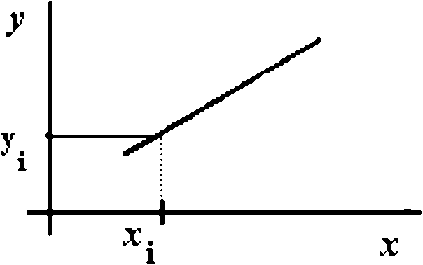
air(y) = Constant = b in the interval (xi, xi+1) with Δxi = xi+1 - xi
Initial Condition
x* = xi ⇒ y* = yi
Figure 2.5 Graphical representation of a simple linear model

|
Properties |
||
|
|
|
|
|
1. |
General expression |
|
|
2. |
Value yI+1 at the end of the interval, Dxi |
|
|
3. |
Variation, Δyi, in the interval, Δxi |
|
|
4. |
Central value,
|
|
|
5. |
Cumulative value,
|
|
|
6. |
Mean value,
|
|
|
|
||
|
Other useful expressions |
||
|
|
|
|
|
7. |
Cumulative value,
|
|
|
8. |
Mean value,
|
|
|
9. |
Mean value,
|
|
|
10. |
Mean value,
|
|
|
11. |
Relation between amr(y) et air(y) |
|
|
12. |
If |
|
|
13. |
In the linear model, the arithmetic mean of yi and
yi+1 is equal to the mean value,
|
|
Important demonstrations
|
General expression Property 1 |
If tia(y) = b in the interval Δxi then y is linear with x and considering the initial condition it will be: y = yi+ b.(x-xi) |
|
Central value Property 4 |
|
|
Cumulative value Property 5 |
from the definition of the cumulative value: it will be necessary to use the factorization of the difference of two squares, that is:
and then:
|
|
Property 10 |
|
Let y = f(x)
Basic assumption of the model
rir(y)=Constant=c in the interval (xi, xi+1), with Δxi = xi+1 - xi
Initial condition
x* = xi ⇒ y* = yi
Properties
rir(y) = air(lny) means that the exponential model of y against x is equivalent to the linear model of lny against x. So being, its properties can be deduced by backwards application of logarithm rules to the properties of the linear model of lny against x.
Figure 2.6 Graphical representation of the exponential model

Figure 2.7 Graphical representation of the linear model of lny against x

|
|
|
Exponential model of y (y against x) |
|
Linear model lny (lny against x) |
|
|
|
|
|
|
|
1. |
General expression |
|
|
lny = lnyi+c(x-xi) |
|
2. |
Value of yi+1 at the end of the interval, Δxi |
|
|
lnyi+1= lnyi+cΔxI |
|
3. |
Variation, Δyi, during the interval, ΔxI |
|
||
|
4. |
Central value,
|
|
|
|
|
|
|
|
|
ln |
|
|
|
( |
|
|
|
5. |
Cumulative value,
|
|
||
|
6. |
Mean value,
|
|
||
|
|
|
|
|
(replacing Δyi using Propriety 3) |
|
|
|
|
||
|
|
|
|
||
|
|
||||
|
Other useful expressions |
||||
|
|
|
|
||
|
7. |
Expressions of variation, Δyi |
Δyi = c.
|
||
|
8. |
Expression of amr (y) |
|
||
|
9. |
Expression of rmr (y) in relation to yi |
|
||
|
10. |
Expression of rmr (y) |
rmr(y) = amr (lny) =
|
||
|
11. |
|
y decreases |
||
|
|
If |
|
|
and vice-versa |
|
12. |
In the exponential model, the geometric mean of yi
and yi+1 is equal to the central value,
|
|||
Demonstrations
Cumulative value
Property 5

Relation between
 and
and

Property 6 - 4th expression
From the approximation
 with h =
c.Δxi
and from property 6-2nd expression, will be:
Finally, by property 4-1st expression, one can conclude that:
