A cohort or annual class or a generation, is a group of individuals born in the same spawning season. The following scheme illustrates the different phases of the life cycle of a cohort:
Figure 3.1 Cycle of life of a cohort
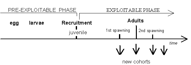
Let us start, for example, with the egg phase. The phases that follow will be larvae, juvenile and adult.
The number of individuals that arrive in the fishing area for the first time is called recruitment to the exploitable phase. These individuals grow, spawn (once or several times) and die.
After the first spawning the individuals of the cohort are called adults and in general, they will spawn again every year, generating new cohorts.
The phases of life of each cohort which precede the recruitment to the fishing area (egg, larvae, pre-recruits), are important phases of its life cycle but, during this time they are not usually subjected to exploitation. The variations in their abundances are mainly due to predation and environmental factors (winds, currents, temperature, salinity,…). In these non exploitable phases mortality is usually very high, particularly at the end of the larvae phase (Cushing, 1996). This results in a small percentage of survivors until the recruitment. Notice that this mortality is not directly caused by fishing.
The recruitment of a cohort during the exploitable phase, may occur during several months in the following schematic ways:
Figure 3.2 Types of annual recruitment to the exploitable phase

With some exceptions, the forms of recruitment can be simplified by considering that all the individuals are recruited at a certain instant, tr called age of recruitment to the exploitable phase. It was established that recruitments will occur on 1 January (beginning of the year in many countries). These two considerations do not usually change the results of the analyses, but simplify them and agree with the periods of time to which commercial statistics are referred.
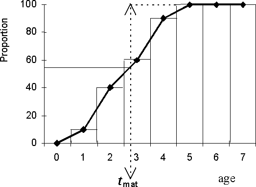
It should be mentioned that not all the individuals of the cohort spawn for the first time at the same age. The proportion of individuals which spawn increases with age, from 0 to 100 percent. After the age at which 100 percent of the individuals spawned for the 1st time, all the individuals will be adult. The histogram or curve that represents these proportions is called maturity ogive.
In certain cases, the maturity ogive can also be simplified supposing that the 1st spawning occurs at the age tmat designated as age of 1st maturity. This simplification means that the individuals with an age inferior to tmat are considered juveniles and those with the same age or older, are considered adults.
Figure 3.3 represents a maturity ogive with the shape of a histogram or curve:
Figure 3.3 Maturity ogive
Consider the interval (ti, ti+1) with the size Ti = ti+1 - ti of the evolution of a cohort with time and Nt the number of survivors of the cohort at the instant t in the interval Ti (see Figure 3.4).
The available information suggests that the mean rates of percentual variation of Nt can be considered approximately constant, that is, rmr (Nt) (constant.
Basic assumption
The relative instantaneous rate of variation of Nt, in the interval Ti is:
rir (Nt) = constant negative = - Zi
Figure 3.4 Evolution of N in the interval Ti
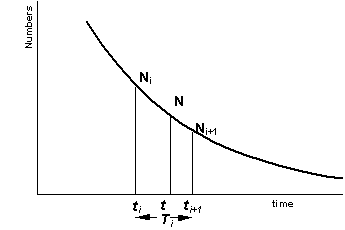
The model of the evolution of Nt, in the interval Ti, is an exponential model (because rir(Nt is constant). This model has the following properties:
Properties
1. General expression. From the basic assumption
rir(Nt) = -Zi
with the initial condition that, for t = ti it will be Nt = Ni then:
2. Number of survivors, Ni+1, at the end of interval Ti
3. Number of deaths, Di, during the interval Ti
(notice that Di is positive but the variation DNi = Ni+1- Ni is negative)
4. Cumulative number of survivors, Ncumi, during the interval Ti
5. Approximate central value, Ncentrali, in the interval Ti
6. Mean number,
 , of survivors during the
interval Ti
when
is small (Zi.Ti < 1)
Comments
1. The basic assumption is sometimes presented in terms of absolute instantaneous rates, that is:
air (Nt) = - Zi.Nt { air (Nt) proportional to Nt} or
air (lnNt) = -Zi
Zi = mortality total coefficient, assumed constant at the interval Ti
Notice that:
+Zi = rir of total mortality of Nt
- Zi = rir of variation of Nt
2. Unit of Zi
From the definition, it can be deduced that Zi is expressed in units of [time]-1. By agreement, the unit year-1 has been adopted, even when the interval of time is smaller or bigger than a year.
The following expressions show, in a simplified way, the calculation of the unit of Zi, with the rules and usual symbols [..(of dimension in the determination of physical units.
3. Annual survival rate, Si
When Ti =1 year it will be:
and also
Si = Annual survival rate in the year i
(or percentage of the initial number of individuals that survived at the end of the year).
1 - Si = Annual mortality rate in the year i
The percentage of the initial number of individuals that die during the year is, by definition, the relative mean rate rmr (Nt) of mortality of Nt, over one year, in relation to the initial number, NI
4. Absolute mean rate

5. Relative mean rate
 in relation to

6. Notice that Si takes values between 0 and 1, that is,
0 ≤ Si ≤ 1 but Zi can be > 1
7. If the limits of the interval Ti were (ti, ∞) then it would be:
Ti = ∞
Ni+1 = 0
Di = Ni
and
The causes of death of the individuals of the cohort due to fishing will be separated from all other causes of death. These other causes are grouped together as one cause designated as natural mortality. So, from the properties of the exponential model, the result will be
rir(Nt) total = rir(Nt) natural + rir(Nt) fishing
Supposing that, in the interval Ti, the instantaneous rates of mortality due to natural causes and due to fishing are constant and equal to Mi and to Fi, respectively, then
Zi = Fi + Mi
Multiplying both factors of the previous equation (equality)
by,  then:
then:
 is the
number, Di, of deaths due to total mortality,
In the same way
 will be the number of dead
individuals due to fishing, that is, the Catch, Ci, in number, and
then:
Notice too that,
 will be the number of dead
individuals due to "natural" causes.
The exploitation rate, Ei, during the interval Ti was defined by Beverton and Holt (1956) as:
and then,or,
The capture in number, Ci, in the interval Ti, can be expressed in the following different ways:
Comments
1. Ricker (1975) defines the exploitation rate, Ei*, as the percentage of the initial number that is captured in the interval Ti, that is: Ei* = Ci/Ni.
a) Ricker’s definition may be more natural, but mathematically Beverton & Holt’s definitions are more useful.
b) It is easy to verify that
2. The exploitation rate, Ei, does not have any unit, it is an abstract number.
3. The possible values of Ei are between 0 e 1, being 0 when there is no exploitation and 1 when the capture Ci is equal to the number of total deaths Di, that is, when Mi = 0.
In order to study the evolution of the biomass of a cohort, one can use the model of the evolution of a cohort, in number, and combine it with a model of the evolution of the mean weight of an individual of the cohort. In effect, the biomass Bt is equal to Nt.Wt where Wt is the individual mean weight at the instant t.
To define a model for the individual growth weight Wt, there are then two possibilities:
ALTERNATIVE 1:
A) To define a model for the mean individual growth in length, Lt
B) To define the relation Weight-Length.
C) To combine A) with B) and obtain a mode for the mean individual growth in weight, Wt
ALTERNATIVE 2:
D) To define directly growth models for Wt and Lt.
ALTERNATIVE 1
A) Model for the individual growth by length
The models that are used in fisheries biology are valid for the exploitable phase of the resource. The most well known is the von Bertalanffy Model (1938) adapted by Beverton and Holt (1957). The existing observations suggest that there is an asymptotical length, that is, there is a limit to which the individual length tends.
Figure 3.5 von Bertalanffy Model
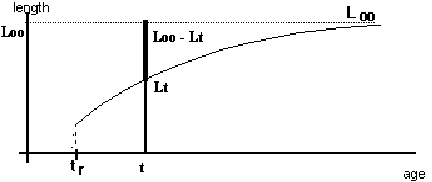
t - age
Lt - individual mean length at the age t
L∞ - asymptotical length
tr - beginning of the exploitable phase
So, Lt presents an evolution where:
air(Lt) is not constant (because growth is not linear)
rir(Lt) is not constant (because growth is not exponential)
However, it can be observed that the variation of the quantity (L∞ - Lt) (which we could call "what is left to grow"), presents a constant relative rate and can be described by an exponential model. So, we can adopt the:
Basic assumption
rir (L∞ - Lt) = - K = negative constant during all the exploited life
where K is the growth coefficient (attention: the growth coefficient K is not the velocity of growth but the relative velocity of what "is left to grow"!!).
The properties of this model can be obtained directly from the general properties of the exponential model. The initial condition:
where ta (and La), that corresponds to an instant within the exploitable phase, will be adopted.
The properties of the model of individual growth by length by
Beverton & Holt (1957) deduced from the exponential model of
 are summarized
as:
|
Properties of the exponential model for |
von Bertalanffy Model for |
|
|
1. |
General expression |
|
|
|
|
|
|
For ta=t0 and La=0: |
For ta=t0 and La=0: |
|
|
2. |
Value at the end of the interval Ti |
|
|
|
|
|
|
3. |
Variation during the interval Ti |
|
|
|
As |
|
|
4. |
Cumulative value during the interval Ti |
|
|
|
|
|
|
5. |
Mean value during the interval Ti |
|
|
|
|
|
|
6. |
Central value of the interval Ti |
|
|
|
|
|
B) Relation Weight-Length
It is common to use the power function to relate the individual weight to the total (or any other) length. Then:
where constant a is designated as condition factor and constant b as allometric constant. This relation can be justified accepting that the percentage of growth in weight is proportional to the percentage of growth in length, otherwise, the individuals would become disproportionate. Thus, the basic assumption is:
where b is the constant of proportionality.
|
C) Combination of A) and B) and comments: |
|
|
1. |
From the combination of
This relation of growth in weight is designated as the Richards equation
(1959). |
|
2. |
From, |
|
3. |
Let |
|
4. |
The Richards and von Bertalanffy models are not the only models used for the evolution of Wt. Other models which have also been used in stock assessment are: Gompertz model (1825) and Ricker model (1969). (see Alternative 2 - property 3) |
|
5. |
Historically, the von Bertalanffy model was developed from the basic assumption Where Cte1 and Cte2 were designated by von Bertalanffy
as the anabolism and the catabolism constants, respectively.
(where Cte1 e Cte2 are other constants). |
ALTERNATIVE 2
D) Model directly for Wt and Lt
In alternative 1, a model was developed for growth in length, and then a model was built for growth in weight, using the relation between weight and length.
The basic assumption adopted by alternative 1 used the
characteristic  instead of
weight in order to be able to have a characteristic with a rate rir constant,
that is, an exponential model. The relation W=a.Lb was adopted to
obtain the model of growth in weight. Notice that it can be said that L was
considered as a function of W, that is, L= (W/a)1/b. It will then be
possible to adopt, instead of that function of W, another function of the
weight,
  in order to be able
to formulate directly the basic assumption:
with the initial condition
Properties
The properties of this model (once it is an exponential model) can be obtained directly from the general properties of the exponential model. It is particularly interesting to derive the general expression Wt resulting from different choices of function H.
|
1. |
General expression |
|
|
|
or |
|
|
2a. |
Richards equation in weight The result will be the general expression: |
Adopting the following function H (Wt) = Wt1/b |
|
|
that is, the Richards equation; and when b=3, this is the equation of von Bertalanffy, so: |
|
|
2b. |
von Bertalanffy equation in weight, will be: |
|
|
3. |
Gompertz equation in weight |
Adopting the function H(Wt) = ln Wt |
|
4. |
The respective equations in length can be obtained by adopting other functions of H(Wt): |
|
|
4a. |
von Bertalanffy equation in length |
Adopting H(Wt) = Lt it will be; |
|
4b. |
Gompertz equation de in length |
Adopting H(Wt) = ln Lt it will be:
|
|
5. |
Simplified equations |
|
|
|
So, the simplified general expression will be reduced to: |
|
|
5a. |
Simplified Richards equation, in weight, will be: |
|
|
|
where t* was represented by t0 because H(Wa) = 0 in Richards model means that Wa will also be zero. |
|
|
5b. |
Simplified Gompertz equation, in weight, will be: |
|
|
5c. |
Simplified Richards equation in length, will be: |
|
|
5d. |
Simplified Gompertz equation, in length, will be: |
|
Comments
1. Gompertz equation, in weight, is similar to Gompertz equation, in length, but, in their simplified forms, t* represents different ages, because they will correspond, respectively, to Wa = 1 and to La = 1.
2. Gompertz equation, in length, is similar to von Bertalanffy if Lt is substituted by ln Lt. In practice, this fact allows the utilization of the same particular methods to estimate the parameters in both equations, using L in the von Bertalanffy expression and lnL in the Gompertz expression. (See Section 7.4)
3. It is important to notice, once again that, in practice,
Lcentrali and Wcentrali are used instead of the mean
values,  and
and

4. Gompertz growth curve in length, has an inflection point, (tinfl, Linfl), with:
tinfl = ta+(1/K).ln(ln(L∞/La)) Linfl = L∞ / e
5. Gompertz growth curve in weight has an inflection point, (tinfl, Winfl) with:
tinfl = ta+(1/K).ln(ln(W∞/Wa)) Winfl = W∞ / e
6. Richards growth curve in length does not have an inflection point but the growth curve in weight has an inflection point, (tinfl, Winfl).
In the particular case of the von Bertalanffy equation it will be:
Winfl = (8/27).W∞ and tinfl = t0+(1/k).ln3
7. Some authors refer Gompertz equation in other ways, for example, using the inflection point tinfl and the asymptotic weight W∞, instead of the parameters ta and Wa.
It will then be or

Sometimes the length expression is presented in its general
form: 
The parameters of the length model will then be: L∞ = a; k = -c et tinfl = (1/c).ln(-b)
8. The growth in length presents an inflection in fish farming, where the study of growth covers very young ages and it is common to use the Gompertz equation. In fisheries, the tradition is to use the von Bertalanffy equation.
9. A model that can sometimes be useful, is the Ricker model (1975). This model is valid for a certain interval of time Ti and not necessarily for all the exploitable life of the fishery resource. In fact, the model is based on the basic assumption that the individual growth is exponential in the interval Ti.
It will be, for example,
 where Ki can be
different from one interval to the next.
1. Biomass
Theoretically, it could be said that the biomass at the instant t of the interval Ti is given by:
Bt = Nt. Wt
Thus, the cumulative biomass during the interval Ti would be:
and the mean biomass in the interval Ti would be:
In the same way, the mean weight of the cohort,
 , in the interval
Ti would be:
The biomass can be obtained by dividing both terms of the fraction by Ti, as
2. Yield
The yield, Yi, during the interval Ti will be expressed as the product of the catch in numbers, times the individual mean weight:
Comments
In practice
 is considered approximately
equal to
  at the interval
Ti.
Other expressions of Yi will also be:
Consider the evolution of a cohort during the exploitable life, beginning at age tr, and intervals of time, Ti, covering all the exploitable phase (frequently the intervals are of 1 year...).
Figure 3.6 illustrates the evolution of the number of survivors of the cohort, N, and the evolution of the catches in number, C, which are obtained during the successive intervals of time Ti.
Figure 3.6 Evolution of the number of survivors of the cohort, N, and the catches in number, C
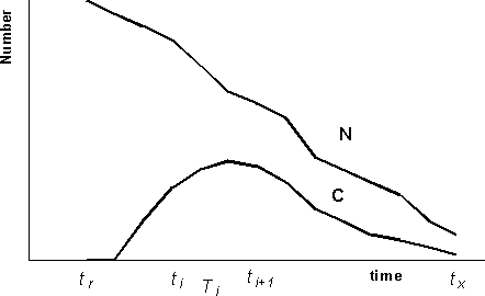
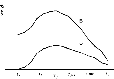
Figure 3.7 illustrates the evolution of the biomass of the cohort, B, and the evolution of the catches in weight, Y, which can be obtained during the successive intervals of time Ti.
Figure 3.7 Evolution of the biomass of the cohort, B, and the catches in weight, Y
Values of the most important characteristics of the cohort, during all the exploitable phase
|
Duration of the life of the cohort |
λ = Σ Ti |
|
Total number of deaths |
D =Σ Di (= R (recruitment) when all the individuals die) |
|
Cumulative number of survivors |
Ncum = Σ Ncumi |
|
Mean number of survivors |
|
|
Cumulative biomass of survivors |
Bcum = Σ
Bcum |
|
Mean biomass of survivors |
|
|
Catch in number |
C = Σ Ci |
|
Catch in weight |
Y = Σ Yi |
|
Mean weight of the cohort |
|
|
Mean weight of the catch |
|
|
Critical age |
tcritique = age where B is maximum, when the cohort is not exploited. |
Comments
1. At first sight it may seem that the values of the characteristics of a cohort during all the exploitable phase are of little interest, because, very rarely is fishing applied to an isolated cohort. At each moment, the survivors of several cohorts are simultaneously present and available for fishing.
2. Despite this fact and for reasons which will be mentioned later, it is important to analyse the characteristics of a cohort during all its exploitable life. Knowledge of the evolution of a cohort, in number and in biomass, and particularly the critical age, is important for the success of the activities in fish farming. As Bt = Nt. Wt, the critical age, tcrítical, will be the age t in the interval Ti where
rir (Wt) = - rir(Nt)=M because, the critical age being the maximum biomass, the derivative of B will be equal to zero.
Notice that Ncum can be expressed in function of the recruitment as
Ncum = R.{...}
where {...} represents a function of biological parameters and annual fishing mortality coefficients Fi during the life of the cohort. Bcum can also be expressed as:
Bcum = R.{...}
where the function {...} also includes growth parameters.
Beverton and Holt (1957) deduced algebraic expressions for the characteristics of a cohort during the exploited life, adopting the simple assumptions:
1. The exploited phase of the cohort is initiated at age tc and is extended to the infinite.
2. The natural mortality coefficient, M, is constant during all the exploitable phase.
Figure 3.8 Life of a cohort during the exploitable phase
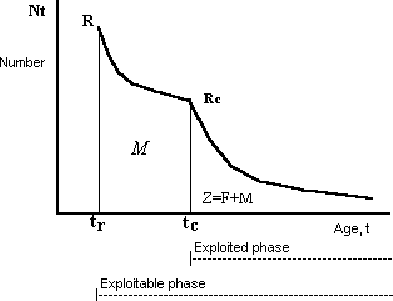
3. The fishing mortality coefficient, F, is constant during all the exploited
phase.
4. Growth follows the von Bertalanffy equation with for La = 0 for
ta = t0
|
1. |
c (ratio between length at age |
|
|
2. |
Recruitment |
|
|
3. |
Cumulative number |
|
|
4. |
Catch in number |
|
|
5. |
Cumulative biomass |
|
|
It can just be written. |
|
|
|
6. |
Mean weight in the catch |
|
|
7. |
Catch in weight |
|
|
8. |
Mean age in the catch |
|
|
9. |
Mean length in the catch |
|
|
10. |
Critical age |
tcritique = |
Comments
1. The simplification of Beverton and Holt allows the calculation of any characteristic of the cohort during its life with algebric expressions, avoiding the addition of the values of the characteristic in the successive intervals Ti. This was useful for calculations in the 60-70's when computers were not available. It is also useful when the only available data is natural mortality, M, and growth parameters.
2. At present, the simplified expressions are also useful to study the effects on the biomass, on yield and on the mean weight of the catch due to changes in the fishing mortality coefficient, F, and/or on the age of first capture, tc. These analyses are usually illustrated with figures. For example, Figure 3.9 exemplifies the analyses of the biomasses and of the catches in weight, obtained from a cohort during the exploited life, subjected to different fishing mortality coefficients, assuming a fixed age tc.
Figure 3.9 Evolution of the biomass and of the catch in weight from a cohort subject to different fishing mortality coefficients and fixed tc (notice that the Figure illustrates only the analysis and does not take into consideration the scales of the axis).
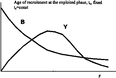
3. Notice that the forms of the previous curves, Y and Bcum against F, do not depend on the value of the recruitment and so, they are usually designated as curves of biomass and yield per recruit, B/R and Y/R, respectively. The calculations are usually made with R=1000.
4. The mean weight, the mean age and the mean length of the catch do not depend on the value of the recruitment. The curves of the characteristics of a cohort during its life against the fishing level, F, or against the age of first catch, tc, deserve a careful study, for reasons which will be stressed in the chapter concerning the long-term projections of the stock.
5. Bcum was calculated as:

where

The calculations can also be made using other values of the constant b, from the relation W-L, different from the isomorphic coefficient, b=3, using the incomplete mathematical function Beta (Jones,1957).
6. The means  and ¯t can be calculated from the cumulative expression


These means are designated as weighted means, being the weighting factors, the number of survivals, Nt, at each age t.