4.1.1 EVOLUTION OF THE AGE STRUCTURE OF THE STOCK
Let us consider the evolution of a stock, with several cohorts, over the period of one year. Figure 4.1 shows the structure of the stock at the beginning of the year, the mean characteristics during the year and the age structure surviving at the end of the year.
Figure 4.1 Structure of the stock at the beginning and end of the year
Let i = 0,1,2,3,... be the ages
4.1.2 CHARACTERISTICS OF THE STOCK AT THE BEGINNING OF THE YEAR
Let:
Ni - number of individuals at age i, at the beginning of the year.
wi - individual weight at age i, at the beginning of the year.
Bi - total biomass of the individuals at age i, at the beginning of the year.
N - total number of survivors of the stock at the beginning of the year.
B - total biomass of the stock at the beginning of the same year.
Then:
4.1.3 CHARACTERISTICS OF THE STOCK DURING THE YEAR
Let:
|
Mi, Fi e Zi |
total mortality (natural and by fishing) coefficients, at age i during the year |
|
|
individual mean weight at age i during the year |
|
|
mean number of individuals during the year |
|
|
mean biomass during the year |
|
C |
catch, in number, during the year |
|
Y |
catch, in weight, during the year |
|
|
mean weight of the individuals caught during the year |
|
|
mean weight of the individuals of the stock during the year |
Then:
(where T=1 year)
(where T=1 year)
with Ncumi, Ci, Bcumi and Yi calculated for all the ages i according to the expressions given previously in Chapter 3 - Cohort.
4.1.4 CHARACTERISTICS OF THE STOCK AT THE END OF THE YEAR
The number of individuals at beginning of age i+1 will be:
Let:
R - recruitment of the cohort in the following year
Then the number and the biomass of the stock at the beginning of the following year will be:
and
where the product R.W1 is the biomass of the recruitment of the following year.
Comments
1. The end of the year coincides with the beginning of the following year. So, the number of survivors of age i at the end of the year will be Ni+1, with age i+1.
2. The sum of the total number of survivors of the stock at the end of the year is not equal to the number of individuals of the stock at the beginning of the following year, because one has to count the recruits entering that year.
3. The total number of deaths, D, during the year,
would be 
4. As the interval of time is 1 year, the cumulative values will be equal to the mean values, that is:
5. The utilization of the same symbols N, B, D, etc., for the stock and for the cohort should not create any confusions.
4.2.1 FISHING LEVEL AND EXPLOITATION PATTERN
The direct action of fishing a stock can be represented by the coefficients of mortality by fishing Fi. These coefficients are associated with the quantity of effort, with the disponibility of the individuals of different sizes or ages, i, and with the fishing gears used by the vessels during the year.
It is usual to separate the coefficients of mortality by fishing into two components:
One is designated as the level of intensity of mortality by
fishing,  , during the year,
called fishing level, F. The level is associated with the quantity of fishing
effort, (the number of vessels fishing), the number of days, hauls, fishing
hours during the year, and with the efficiency or the fishing power of the
vessels or gears. Another component, designated as exploitation pattern,
si, is associated with the selective properties of the fishing gears
relative to the sizes or ages of the individuals available to be captured,
during that year.
The combined set of the fishing level (a unique value for all ages) and the exploitation pattern (different values according to the size or the age), is designated as fishing pattern or fishing regime. The designation of fishing pattern may cause some confusion with the exploitation pattern, and the designation of fishing regime may be confused with what the economists and managers call fishing regime.
The fishing pattern, Fi, of one age i during one
year, is equal to the product of the fishing level of that
year, , times the
exploitation pattern of each age, si. That is:

To analyse the effects of the coefficient of mortality by
fishing,  , on the
characteristics of the resource and on the catches, the exploitation pattern is
generally taken as constant from one year to the next. Sometimes one analyses
the effects of the changes of the exploitation pattern maintaining a fixed
fishing level, but one can also analyse the combined effects of the two
components.
The fishing level,
 , is often represented by
F.
Knowing the structure of the stock at the beginning of one
year, it is possible to estimate the characteristics of the stock during that
year and project the structure of the stock for the beginning of the next year
(with an exception to the recruitment of that year), for different values of the
fishing level,  , (and for
the exploitation pattern, si).
It is, of course, necessary to know the biological parameters of growth, maturity and the natural mortality coefficients, in each age during the year.
Adopting one value for the recruitment of the following year, the projection could be repeated for one more year and so on. The inconvenience in projecting the stock for several years will be that those projections will depend more and more on the adopted annual recruitment values. That is why, in practice, the stock and the catches are projected for one, or at the most, two years. In Section 4.5, the estimation of recruitments will be discussed.
Notice that to project a stock for the following year, it is necessary to have data from the previous year. So, the stock is firstly projected for the current year and then the catch and the biomass are projected for the following year.
Let us suppose, for example, that in 1997 one wants to project the characteristics of the stock for 1998. As the available data will be, in the best hypothesis, referring to 1996, one will have to project the stock of 1996 for the beginning of 1997 and together with the recruitment of 1997, project the stock until the end of 1997 and only after that, can one project to 1998, estimating previously the recruitment of 1998.
Let us consider the vector N with the components N1, N2,..., Ni,... representing the structure of the stock at the beginning of a year. Notice that N1, N2,..., Ni,... are the survivors of the different cohorts of the stock, at the beginning of the year.
Let Mi and Fi be the natural and fishing mortality coefficients of age i, assumed to be constant in the future years.
Figure 4.2 illustrates, with a theoretical stock, the projections of the numbers of survivors of the different cohorts at the beginning of 1980, for the years to come, from 1981-1986 (the values are expressed in million of individuals).
Notice that the recruitments are missing during the years 1981 to 1986, as they have not yet occurred. So, it is clear that the respective survivors are also missing during those years.
Let us suppose now that the recruitments of the same period of years were equal to those of 1980, that is, 440 million of individuals. Figure 4.3 shows the projections in future years. It can be seen that the values of the age structure of the stock in 1986 are equal to the annual evolution of the cohort in 1980.
Figure 4.2 Structure of the stock at the beginning of 1980 and projections of the number of survivors (million of individuals) of the different cohorts at the beginning of the years 1981-1986

Figure 4.3 Long-term projections of the cohort of 1980 and structure of the stock assuming a constant annual recruitment of 440 million of individuals

One practical conclusion seems to be that to obtain the structure of the stock in 1986 it would be enough to follow the evolution of the cohort of 1980 and then, it would not be necessary to have the complete structure of the stock at the beginning of the year. It would be enough to adopt one value for the recruitment (R) of a cohort (and, of course, assume that the biological parameters would be stable in the following years). An advice would be to make the calculations adopting a Recruitment of 1000 individuals (with computer software a recruitment equal to 1 is adopted).
Except for the mean values - age, length, weight in the catch, etc, - which are independent of the adopted value of R, the characteristics of the stock in the long-term, under the previous conditions, are proportional to the recruitment. So, these projections are also designated as projections by recruit, by LT projections or even as equilibrium projections.
The long-term projections do not only concern the survivors at the beginning
of the year, but also the values of the mean abundances,  during the year, and the catches in number, Ci.
One can also project the total biomasses, B or
 , the spawning biomasses, SB
or
  , as well as the catches
in weight, Y, knowing the initial individual weights, Wi, the mean
weights,
  , and other
parameters like those of maturity.
It is important to verify that the cumulative values,
Ncumi e Bcumi, of a cohort during 1 year are equal to the
mean values,  e
e , during that year. The
long-term projections can be calculated as:
(
)
Several long-term projections can be made with different
values of Fi, that is, with several fishing levels,
 , and/or with several
exploitation patterns, si.
As mentioned before, the analyses of the effects of the fishing pattern on the catches and stocks can be done with the two components (fishing level and exploitable pattern), separated or combined.
Figure 4.4 (A-C) illustrates several types of yield per recruit curves, maintaining a fixed exploitation pattern. The curves are different for other exploitation patterns.
Figure 4.4 Examples of types of curves of the Yield per Recruit (Y/R) against F, given the exploitation pattern: (A - with a maximum, B - flat-top, C - asymptotic)

Figure 4.5 (A-E) illustrates the relations between the most important characteristics of the stock and fishing level, maintaining a stable exploitation pattern:
Figure 4.5 Relations between the long-term characteristics of the stock against the fishing level F, (A - mean number/R, B - catch in number/R, C - mean weight in the catch, D - mean biomass/R, E - yield/R)

A more detailed analyses of these curves will be presented later on, in Chapter 5.
Conclusion
|
The long-term structure of the stock by ages during 1 year |
= |
Evolution of the cohort during its life |
Comments
|
1. |
One projects a cohort during its life in order to obtain the long-term projection of the stock for one year, assuming the annual recruitments to be constant. |
|
2. |
It is necessary to know Mi for all ages of the cohort, as well
as Wi, |
|
3. |
Any recruitment size can be used. Adopt R = 1000 (or R = 1) with worksheets on your computer. |
|
4. |
The five most important characteristics of the stock are
|
|
5. |
A characteristic of the stock that is also important is the spawning biomass, SB. To calculate SB, it is necessary to know the maturity ogive (or histogram). |
|
6. |
Long-term projections are also designated as equilibrium situations. |
|
7. |
Long-term projections are useful to define the long-term management objectives. |
|
8. |
Annual
|
|
9. |
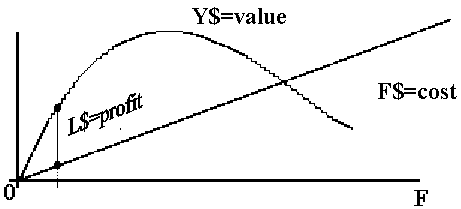
Economists transform the total yield, Y. into value Y$,
the mean weight of the catch,
|
Figure 4.6 Long-term relations between the value of the catch, the cost of exploit- ation and the profit against the fishing level
The stock-recruitment relation, known by S-R relation, associates the size of the stock, for one year, with the recruitment which results from the stock spawning normally during that year. The recruitment can be the recruitment at the exploitable phase and the stock can be the spawning stock. This recruitment may occur one or more years after the spawning.
The problem with the relation between the parental population and the new generation is not a special case of the fisheries resources, it is common to all the self renewable populations.
It is important to determine, in each case, the stock and the recruitment to be used. In fact, that stock can be the total number of individuals (at the beginning of the year or the mean value during the year), the number of adult individuals of the stock, the number of adult females, etc. One can also adopt, not the abundances in number, but the corresponding biomasses. The decision will depend on the type of resource and on the available data. It is necessary to define if the recruitment is in weight or in number and if the recruitment is to the fishing area or to the exploited phase.
In this manual, stock (S) will be considered as the spawning biomass and the recruitment (R) will be expressed in number.
After the spawning, the individuals of the new generation will have to go through different phases of the biological cycle: eggs, larvae and juveniles, before they become recruits. These phases, which, in some species can take years, are not directly submitted to the fisheries exploitation. That is why fishing in those years does not directly affect the size of the new recruitment. It is true that fishing acts on the size of the parental biomass, but that does not happen in the pre-recruit phases, and it is precisely for that interval of time that the relation S-R is applicable.
There is, in these pre-recruit phases, a great mortality due to climate and environmental factors (winds, currents, temperatures, etc.) as well as due to biological factors (available food, predation and others).
A great variety of factors (besides fishing) cause great fluctuations to the recruitment sizes, therefore, the relation S-R is a complex one. In conclusion, the relation S-R, between the stock and the resulting recruitment, can be considered independent of fishing.
Figure 4.7 Example of the dispersion of the points in the relation S-R
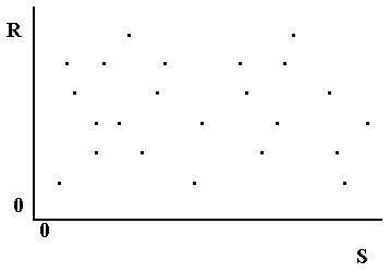
Figure 4.7 shows the type of dispersion of values in the plot of recruitment (R) against parent stock (S).
Despite the difficulties, some models have been proposed for the relation S-R. One of the reasons for this is that there must be a relation. One point of the relation (S = 0, R = 0) is even known already.
4.5.1 BEVERTON AND HOLT MODEL (1957)
Beverton and Holt, when analysing plaice fishery in British waters proposed one model, which can be re-written as:
where α and k are constants.
Figure 4.8 Beverton and Holt Relation S-R
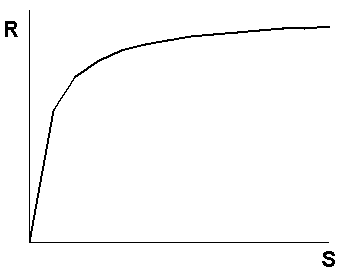
This model shows a curve where R is asymptotic when S → ∞.
4.5.2 RICKER MODEL (1954)
Ricker, studying cod fishery in Canadian waters proposed another model that can be written as:
R = α.S.e-S/k
where α and k are constants.
Figure 4.9 Ricker Relation S-R
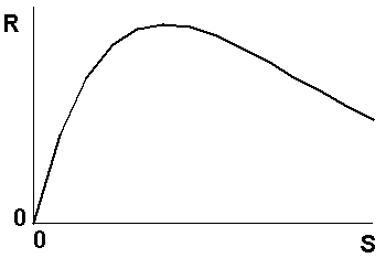
This model presents a maximum resulting recruitment at an intermediate value of the parental stock, S.
4.5.3 OTHER MODELS
Other models of S-R have been proposed, like the Deriso generalized model (1980), which can be re-written (Hilborn & Walters, 1992) as:
(the model is the Beverton and Holt for c = -1 and when c → 0 it is the Ricker model)
or Shepherd's generalized model (1982), as:
(the model is the Beverton and Holt when c = 1 and when c = 2 the curve is an pproximation of the Ricker model)
Notice that in every model presented, S=0 implies R=0, as expected and the slope of the tangent to the curve at that point, (0,0), is equal to the parameter α. Sometimes, the relations S-R are presented as R/S in function of S, so the Beverton and Holt equation would be:
showing that the inverse of R/S is linear with S.
With the Ricker model the relation between R/S against S would be:
that is, R/S is exponential negative with S (or ln(R/S) is linear with S).
With the Deriso model it would be (R/S)c linear with S.
Mathematically, these linear relations can be useful to estimate the parameters α and k, but statistically they cause some problems, because the variable S appears in the response variable and in the auxiliary variable.
Comments
1. Remember that relations S-R are independent of the fishing level.
2. Relations S-R may be introduced in the calculations of the stock projections. In that case, the projections will have to be made every year and they will require the structure of the stock at the beginning of the initial year.
3. It must not be forgotten that there is a great dispersion of the observed points (S, R) around the model.
4. To determine the limit of the Deriso equation when c → 0 it is enough to remember that limit (1+A/n)n = eA when n → ∞ and A is a constant.
5. The Beverton and Holt model presents an asymptote, R → α.k when S → ∞. When S=k it will be R = α k/2.
The Deriso model presents the maximum:
Smax = k / (1+c), Rmax = α.k / (1+c)1+(1/c)
The Shepherd model presents the maximum:
Smax = k.(c-1)-1/c, Rmax = (α/c).k.(c-1)1-(1/c)
 (R-S
RELATION)
(R-S
RELATION)Up to now the discussion have been centred on the relation S-R, that is the relation between the biomass S and the resulting recruitment R. There is another relation (which has already been referred to in Section 4.4 Long-term projections of the stock, particularly in the conclusion about the structure of the stock and the evolution of a cohort during all its life) that could be called the relation R-S, that is the relation between the recruitment R and the resulting cumulative biomass, Bcum of a cohort during all its life for a given fishing pattern.
The cumulative biomass (or spawning biomass) of a cohort during its life, Bcum, is, as it has already been seen, equal to:
Bcum= R. {function of biological parameters and of the fishing pattern, F}
As mentioned before, the cumulative biomass, Bcum,
of a cohort during its life is equal to the long-term mean biomass,
 , of the stock during
one year, so, one can refer to the Bcum as
 .
.
It can then be said that in the long-term, if the biological parameters are considered constant, then for a certain fishing pattern, the mean biomass of a stock during one year is proportional to the recruitment. Figure 4.10 illustrates the proportionality.
Figure 4.10 Illustration of the
proportionality in the long-term between the mean Biomass
 of a stock and the
Recruitment (R), for a certain fishing level, F, assuming that the exploitation
pattern and the biological parameters are constant

Notice that in Figure 4.5-D, the relation B/R against F was shown. The two curves 4.5-D and that of Figure 4.10 are different representations of the same situation. While in Figure 4.5-D, a value of F corresponded to a value of B/R given by the curve, in Figure 4.10 the value of F will correspond to a slope B/R of a given straight line.
For other values of F, the straight line of Figure 4.10 will have different inclinations. Figure 4.11 shows several lines according to the different values of F.
Figure 4.11 Illustration of four lines corresponding to different fishing levels, F
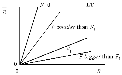
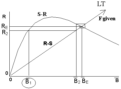
Figure 4.12 shows the overlapping of the Ricker curve S-R (Figure 4.9) and the line in Figure 4.10, the axes of this last figure having been switched. To avoid confusions, it is convenient to refer the slope of the line corresponding to a value F in relation to the axis R.
Figure 4.12 Overlapping of the curve S-R with the line R-S for a given F

One can start from a value of biomass, and, through the
relation S-R, determine the future recruitment, R. That R will give a resulting
biomass, , through the
straight line. This process can be repeated until a situation of equilibrium is
found.
It will be possible to illustrate the combined analysis through the two relations for a certain fishing level.
For example, let us select one value
 . The curve S-R allows the
calculation of the resulting value R2. Through the line (of a given
F), the resulting value of
 will correspond to that
value of R2, and so on. Figure 4.13 shows that the process reaches
the equilibrium point (RE,
 ). This point would
correspond to a value of the fishing level F, determined by the slope of the
line in relation to the R axis.
Figure 4.13 Illustration of the
process that, starting from a biomass
 , theoretically leads
to the equilibrium point (RE, BE)
Notice that the intersection of the two relations does not always lead to an equilibrium point. The existence of an equilibrium point depends on the angle between the straight line and the curve at the intersection point.