2.1.1 Introduction
2.1.2 Functions
2.1.3 Powers and logarithms
2.1.4 Derivatives
2.1.5 Integrals
In the analysis of a fishery and in stock assessment one is mainly interested in changes. They can be changes in the number of a stock with time, changes in weight of a fish with age, changes in yield with changes in the fishing effort, etc.
Changes with time are measured as rates, i.e. the change in the magnitude of the quantity (weight, etc.) considered divided by the period of time during which it occurred. Even if the time interval is not explicitly specified, unit time (e.g. one year) is usually to be inferred and thus the change is implicitly a rate.
In mathematical terms, if for a period of time D f, a variable y changes by the amount D y, then the mean rate of change during this period is D y/D t. This rate is an absolute rate. A relative rate can be obtained by dividing the absolute rate by the value of the variable at some point during the period, e.g. at the beginning, when it becomes  . These concepts can be generalized taking t as any variable, not necessarily time.
Theoretical models have the advantage of permitting the analysis of the influence of some factors by studying the mathematical properties of the models. For mathematical simplicity in these models and elsewhere instantaneous rates are often used.
Instantaneous rates can be taken as the limit of the mean rates when the period of time, D t, tends to zero. Mathematically this is equivalent to the concept of the derivative.
The hypotheses to be made on the relationships between instantaneous rates and the variables can be expressed in the form of differential equations. The differential and integral calculus are important mathematical tools in the analysis of the dynamics of population and other systems. Some of these hypotheses lead to the exponential, logarithmic and power functions.
For the above-mentioned reasons a quick review of powers, exponential and log functions, as well as of differential and integral calculus, is important. Granville, Smith and Longley's Elements of the differential and integral calculus deals extensively with such matters.
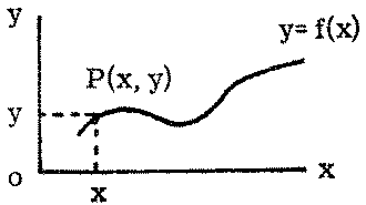
Let x and y denote two variables. If to each value of x corresponds a value of y then we can say that y is a function of x or symbolically y =f (x). Graphically, if we plot the values of x on the abscissa (horizontal) axis and the corresponding values of y on the ordinate (vertical) axis, the curve joining the points, P (x, y), with abscissa x and ordinate y, is a graphical representation of the function y = f (x):
FIGURE 2.1.
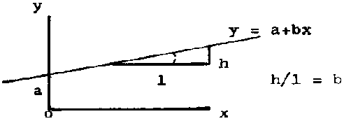
Perhaps the simplest and one of the most used functions is the linear function y = a + bx where a and b are constants. Its graphical representation is a straight line with the intercept on the axis of y equal to a and the slope equal to b:
FIGURE 2.2.
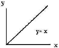
When a = 0 then y = bx, which represents a straight line passing through the origin. This relationship states that y and x are directly proportional (Figure 2.3.1). For the special case b = 1, the equation y = x is the bisector of the positive quadrant (Figure 2.3.2).
FIGURE 2.3.1.
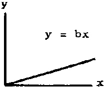
FIGURE 2.3.2.
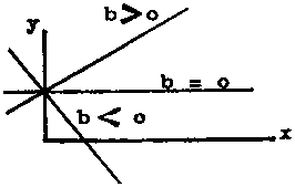
The figure below shows the position of the straight line for different values of b
FIGURE 2.4.
Another way of writing the linear function is:
y - y0 = b (x - x0) where (x0, y0) is one point of the line.
This form is especially useful when we know two points of the line and we wish to formulate the equation. Thus, if one point is (x0, y0) and the other is (x1, y1) the line will pass through both if b satisfies the equation y1 - y0 = b (x1 - x0), that is, b = (y1 - y0)/ (x1 - x0). The equation can then be written immediately.
In a linear function the mean absolute rate of change of y with x is constant and equal to the slope. Thus the instantaneous absolute rate is also constant and its value is the slope b.
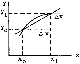
For any other function the mean absolute rate between two values x0 and x1, is the slope of the straight line passing through the points (x0, y0) and (x1, y1)
FIGURE 2.5.
Another very useful function is the parabola, also called the second degree polynomial, y = a + bx + cx2
FIGURE 2.6.
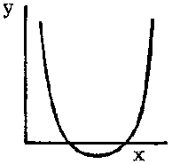
The equation can sometimes be written in the form: y = A (x - x0) (x - x1) where x0 and x1 are the intercepts on the x-axis and the sign of the constant A determines whether it is concave upward or downward.
FIGURE 2.7.1.
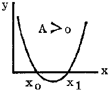
FIGURE 2.7.2.
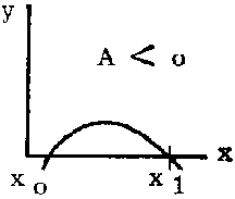
FIGURE 2.7.3.
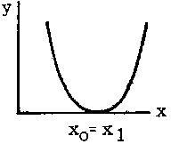
The exponential function y = ax where a is a positive constant has the graphical representation shown in Figures 2.8.1 and 2.8.2.
FIGURE 2.8.1.
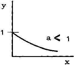
FIGURE 2.8.2.
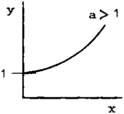
An exponential function commonly used for its mathematical convenience is the one with a equal to the mathematical constant e.
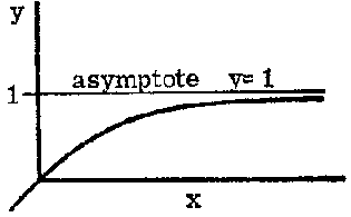
Some curves have an asymptote, i.e. a straight line to which the curve approaches closer and closer as x becomes extremely large (or extremely small); more precisely they are tangents to the curve when x = ¥ (or - ¥). For example: y = ax with a < 1 (see Figure 2.8.1) has the asymptote y = 0; the curves y = 1 - e-2x and y = 1 - e-2x both have the asymptote y = 1, the second one approaching this asymptote rather more quickly.
FIGURE 2.9.
The representation of the relationship between two variables may often be simplified by transforming one of the variables, i.e. by using some function of the variable rather than the variable itself. Thus if we are considering the relation: y = A/x, this may be transformed into a direct proportional relationship using the variable  , then y = Aw.
It is always possible to transform a mathematical function into a straight line relation by a suitable transformation of variables. This is often useful when fitting a theoretical, and possibly complicated curve to observed data; the fitting of a straight line, either graphically by eye, or by regression techniques is relatively simple. Fitting more complex curves, e.g. the exponential, is more difficult, either by eye or by calculation. It should be noted that the least square regression (or other fitted curve) which uses the arithmetic means of the transformed variables will probably not coincide with the arithmetic mean of the original variables, e.g. using the transformation w = log x, the arithmetic mean of the w's is the geometric mean of the x's.
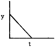
As we will see later, the curve relating the number of fish of a year-class alive at time t can be expressed as Nt = N0e-Zt and can be transformed into the straight line y = a + bt, where a = logeN0 and b = - Z, using the logarithmic transformation y = logeN.
FIGURE 2.10.1.
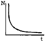
FIGURE 2.10.2.
The functional relationship y =f (x) can also be expressed in the inverse way, that is expressing x as a function of y, x = g (y). For instance, the linear relation y = a + bx can be expressed in the inverse form (also linear)  (provided b ¹ 0). If the function f (x) is other than a simple linear one, it may happen that more than one value of x will give the same value of y; then the inverse function x =g (y) will not be a simple single valued function. For instance, if y = x2, then the inverse function is
  . Graphically, the representation of a function and its inverse are identical. Given a graph of y =f (x) this can be used as a graph of x = g (y) by a simple interchange of axes.
A power is represented by two numbers and written symbolically as an, where the number a is called the base and n the exponent. When the exponent is a positive integer, an is defined as the product of n factors each equal to a; when the exponent is 0, then a0 is defined as equal to 1; when the exponent is a fraction, let us say  , then by definition
  ; when the exponent is negative, let us say - m, then by definition
  .
.
When the base is positive the power is positive, but when the base is negative the power is positive if the exponent is even and negative if the exponent is odd.
It is useful to consider the value of a power when the exponent n increases without limit.
If the base a is greater than 1 then an also increases without limit.
If the base a is equal to 1 then an is equal to 1 for all values of n.
If the base a is smaller than 1 (and positive) then an tends to 0.
Some useful rules for multiplying or dividing powers are:
- Powers with the same base

- Powers with the same exponent

To raise a power to an exponent, the base is raised to the product of the exponents:
(an)m = anm
The function y = an can be considered in two ways depending on whether the base a, or the exponent n is considered as the variable of interest. In the form y = xn (i.e. the base is the variable) it is called a power function; in the form y = ax (i.e. the exponent is the variable) it is called an exponential function.
The inverse function of a power is a root and the inverse function of an exponential is a logarithmic function. Thus if y = ax then x = logay, or x is the logarithm of y to the base a.
When the base is the constant e, the logarithms are called natural or Napierian (or hyperbolic).
From the definition above one can see that the properties of the powers will imply corresponding properties of the logarithms, e.g.
loga (A · B) = loga A + loga B corresponds to the property ax · ay = ax+y

loga (Am) = m loga A corresponds to the property (ax)y == axy
Special relations can also be obtained, such as loga 1 = 0 and loga a = 1. The relation between the logs of a number on two different bases, a and b, is:
loga N = logb N · loga b
The bases most used for logs are the base 10 and the base e (e » 2.72), the former because 10 is the basis of the numerical system currently used and the latter because this results in the most simple form of several mathematical relationships. From the above relation the logarithm of a number to the base e can be obtained from the logarithm of the number on base 10 multiplied by loge 10 ~ 2.303. This is a useful expression if a table of natural logs is not available. One of the advantages of using the base 10 is that any number can be expressed as the product of a power of 10 and a number between 1 and 10, e.g. 283.5 = 102 × 2.835; 0.0053 = 10-3 × 5.3. In this way the decimal log of any number will be the sum of the decimal log of a number between 1 and 10 (mantissa) plus the decimal log of a power of 10, that is, its exponent (characteristic).
From the above examples this would give log10 283.5 = 2 + log10 2.835 and log10 0.0053 = -3 + log10 5.3. The logarithms to base 10 of the numbers between 1 and 10 are given by tables.
Tables of natural logarithms are usually available over a wider range (perhaps from 0.1 to 100) but natural logarithms can be obtained by a similar method for any range from tables of the natural logarithms from 1 to 10. For instance,
loge 283.5 = 2 loge 10 + loge 2.835 = 2 × 2.303 + 1.042 = 5.648 andloge 0.0053 = - 3 loge 10 + loge 5.3 = - 3 × 2.303 + 1.667 = - 5.242
As already stated, the concept of derivative is equivalent to the absolute instantaneous rate and this is the limit of the absolute mean rate during an interval when the length of the interval tends to zero.
Let us consider a function y = f (x). If x is given an increment D x, y will have an increment D y. The limit of the quotient of the increments,  , when D x tends to zero will be the derivative of y with respect to x at the point (x, y). This can be represented by the symbols
  or y' or f' (x).
Graphically, the incremental ratio  is the slope of the secant to the curve passing through the points (x, y) and (x + D x, y + D y) and the derivative
  is the slope of the tangent to the curve at the point (x, y) (the tangent is the limit of the secant when D x tends to zero and x + D x tends to x).
FIGURE 2.11.1.
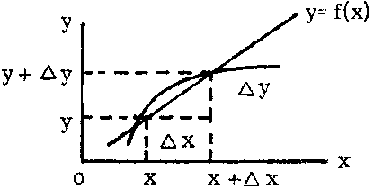
FIGURE 2.11.2.
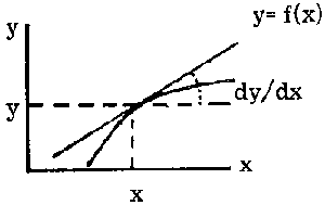
Thus derivative, absolute instantaneous rate and slope of the tangent are equivalent concepts expressed from different viewpoints. Using this definition, we can calculate the derivative of a function. For instance, to determine the derivative of y = 3x2 we can start by calculating the increment of y for a given increment of x. We obtain the value of the function at the point x + D x and subtract from the value of the function at the point x:
|
at x |
y = 3x2 |
|
at x + D x |
y + D y = 3 (x + D x)2 = 6xD x + 3D x2 |
|
then D y = 6xD x + 3D x2 | |
The incremental ratio will be  . As D x becomes very small, the second term on the right will also become small and in the limit as D x ® 0 this second term also tends to zero, so that
  will be equal to 6x.
Derivatives can be arrived at easily if we obtain, in that way. some rules, e.g.
Derivative of a constant, c, is zero:
Derivative of a variable x with respect to itself is:
Derivative of the product of a constant c and a function u (x) is the product of the constant and the derivative of the function:
Derivative of a sum of two functions, u (x) and v (x), is the sum of their derivatives:
Derivative of a product of two functions, u (x) and v (x), is given by
Derivative of a power of a function u (x) is given by
Derivative of the quotient of two functions, u (x) and v (x), is given by
We can also obtain from further analysis the derivative of special functions often used in fisheries studies, such as
(ex)' = ex(eu)' = euu'
It is interesting to note that the derivative of the function ex is ex itself; it is this property of the exponential of base e which makes it so important on theoretical grounds.
The derivative of the function y = eax is y' = eaxa = ay; this means that the derivative, or the instantaneous rate, of y is proportional to y, a property very useful in many situations (e.g. studies of growth, mortality, etc.).
As an example of how we could apply these rules let us calculate the derivative of y = (3 + e2x) (1 - x2).
Applying the rule for a product we can write
To calculate the derivative of the first factor we can apply the rule concerning the sum of two functions, then (3 + e2x)' = (3)' + (e2x)'. We thus see that (3)'= 0 and (e2x)' = e2x (2 x)' = e2x · 2 and thus (3 + e2x)'= 2e2x. Calculating the derivative of the other factor: (1 - x2)' = (1)' - (x2)' = 0 - 2x = - 2x. Finally y' = 2e2x (1 - x2) - 2x (3 + e2x).
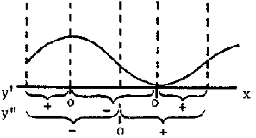
The derivative of a function of x is, in general, another function of x. This function may also be differentiated to give another function of x. This last is called the second derivative of the original function. It is usually represented by the symbols y¢ ¢ or d2y/dx2 and could be interpreted as the absolute rate of the absolute rate, which in physics is called acceleration. Third, fourth, etc. derivatives can also be defined.
An application of the first derivative is the analysis of the change of a function and of the second derivative the analysis of the rate at which this change is itself changing. For the points where y' is positive, y is increasing, and where y' is negative, y is decreasing. If y' = 0, y is a stationary point. When y¢ ¢ is positive the slope of the curve is increasing and the graph of y is concave upward; when y¢ ¢ is negative the slope of the curve is decreasing and the curve is concave downward. If y¢ ¢ = 0, y is an inflection point (unless y' was also 0). From the sign of y¢ ¢ we can decide if the stationary points are maxima or minima.
FIGURE 2.12.
In the last section we saw how, given a function, we could obtain its derivative. The reverse problem would be to obtain the function knowing its derivative. This operation is called integration and the function so obtained is called the integral. For instance, what is the integral of 3x2? We have seen that the derivative of x3 is 3x2, thus an integral of 3x2 could be x3. But so also is x3 + 4 or generally x3 + C where C is any constant, since the derivative of a constant is zero. This means that the integration of a function does not produce a simple function but a family of functions defined by the additive, arbitrary constant C.
The integral of f (x) is represented by  or F (x) + C and is called the indefinite integral. It is indefinite because of the arbitrary constant C.
The rules of integration can easily be obtained from the rules of differentiation, as they are inverse operations. Thus
Useful expressions are
A technique very useful for integration is the change of variable. For instance to integrate e4x-3 we can put v = 4x - 3 and dv == (4x - 3)' dx or dv = 4 dx. Then
If one knows a value of the integrated function it is possible to determine the corresponding value for the constant C. In general terms we can say that if y = F (x) + C is the integral of a function, and knowing that (x0, y0) is a point of the integral curve then y0 = F (x0) + C and C = y0 - F (x0); thus y - y0 = F (x) - F (x0) gives the curve which satisfies the conditions of the problem.
We have seen the integration as the inverse operation of differentiation. There is however another concept of integral. This concept can be easily understood through the calculus of areas, which is one of the most important applications of integrals. Let us, for instance, calculate the area under the curve y =f (x), the axis of abscisses and the ordinates at x = a and x = b.
FIGURE 2.13.
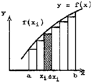
This area can be approached by the sum of the areas of the rectangles of base D xi, and height f (xi), this is S f (xi)D xi, where the interval from a to b was subdivided in n small intervals D xi. The limit of this sum when the number of subdivisions increases indefinitely and each interval decreases to zero can give the area required. This limit is then the definite integral. This definite integral, g (x) is one possible value of the indefinite integral, since the rate at which the area under curve increases as x increases is equal to the height of the curve, so that  . The area under the curve between x = a and x = b is written
To calculate the definite integral we calculate as before the indefinite integral and subtract its value for x = b and for x = a, this is:
As an example let us calculate the area under the function y = 3x2 + 5 between x = 2 and x = X.
(Note that when calculating geometrical areas the values of the function and of its integral must be taken as positive.)
Another very important application of integrals is in solving differential equations. A differential equation is an equation with derivatives or differentials, for instance, y' = 4 x - 1 or dy = (5 + 2x) dx.
Differential equations can be very difficult to solve, but some elementary processes are applicable to easy equations. One of these processes is called the separation of variables. For instance, let us integrate the equation dy = xydx. By a simple operation we can obtain (separate) all the expressions with the variable y in a member of the equation dy and the expressions with the variable x in the other:  .
.
Now each member can be integrated separately:
or  or, joining the arbitrary constants,
The same result could be presented in a slightly different way by, instead of the constant C, using arbitrary point (x0, y0), thus

and
This last expression can be very useful when one is interested in pointing out some special point of the function.
Fish population studies involve the measurement and analysis of many quantities - e.g. age compositions, and growth rates - few of which can be measured exactly, either because of their inherent variability or the difficulty of measurement. Statistics must therefore be used to some extent, if only in such a simple form as taking the mean of a set of values. Basic statistical methods are the same whatever the subject in which they are being applied, and are described in many textbooks. These notes will therefore only deal very briefly with the basic methods. Some applications, e.g. correlation and regression analysis will be dealt with later as they occur. In this section most attention will be paid to the problem of sampling fish populations. (Statistics is dealt with in more detail in another manual in this series, in which both the basic methods and special applications to fisheries are described.)
In statistics we are concerned not so much with any individual value, e.g. the size of any one particular fish on the fish market, but with the frequency with which the various values (e.g. size of fish) occur. Such frequency distributions may be represented graphically, either as histograms or frequency polygons. Much of the frequency distributions can be described by two quantities; the average value (or the position of the curve) and the spread. The most common measures for the average are the arithmetic mean (or simply mean), the median (or half way value) and the mode (or most frequent). Of these the mean has most advantages. The common measure of dispersion is the variance, which is the average of the square of the deviation from the mean; the square root of the variance is the standard deviation. Further discussions of these measures, together with methods of calculation etc. may be found in most textbooks, e.g. Yule and Kendall (1950), chapters 4, 5 and 6.
Tests of significance are another group of statistical tools of great use in fishery research, as in most other fields. While the explanation of the arithmetical steps involved in any particular test will be left to the appropriate section of the textbooks, e.g. Yule and Kendall (1950), chapter 21, it is worth emphasizing here the underlying basis of tests of significance. That is, we assume some null hypothesis, and on this basis calculate the probability of the observed values occurring. If this probability is sufficiently small (usually one in twenty, or one in a hundred) we reject the null hypothesis. For instance, using the t-test for the difference in the means of two samples, the null hypothesis is that the two samples come from the same population. If the probability of a value of t equal to or greater than that observed occurring is say 0.01, this means that if the two samples had come from the same population, an unlikely event (a one in a hundred chance) has taken place and we therefore believe that the two samples did not come from the same population, i.e. they are statistically different. Such a test does not give any information on the probability of the two samples coming from different populations, or on the practical significance of the difference. For instance, two small and variable samples may differ by an amount which is not statistically significant, but which if real would be most important. Conversely, for two large and homogeneous samples a difference may be large enough to be statistically significant, but yet so small as to be negligible in practice.
2.3.1 General
2.3.2 Sampling the landings
2.3.3 Sampling the population
(For further details see FAO. Manual of sampling and statistical methods for fisheries biology, by J.A. Gulland. Part 1. Sampling methods. Rome, 1966.)
Most of the quantities involved in fish population work cannot be obtained or measured throughout the whole population; e.g. it is virtually impossible to measure all fish caught, even less all the fish in the sea. A section, or sample, of the whole population is therefore examined for the attributes concerned, e.g. percentage of mature fish, or average size. On the assumption that this sample is representative of the whole population, an estimate may be made of the true value in the population. If the sampling system used is a good one, then the estimate obtained will differ little from the true value. The merits or otherwise of a sampling system can therefore be measured by two quantities relating to the estimates obtained (those measures refer not to any individual estimate, but to the set of estimates which might be obtained by repeated samples); firstly, the variance, which as defined above for any statistical distribution, is the measure of the scatter of the estimates about their mean value; secondly, the bias, which is the extent to which the mean value of the set of possible estimates differs from the true value. (The term bias is also used for the processes leading to this difference.)
Because when a bias exists, it exists in all samples, tending to make the estimates constantly greater (or less) than the true value, it cannot be detected as a difference between repeated samples; thus in general bias is very difficult to detect, and hence eliminate, in subsequent analysis. A large variance, in contrast, appears at once in the differences between samples. Large bias is therefore even less desirable than large variance, in that it may cause what appear to be reliable and consistent data to give results that are consistent only in the extent to which they are wrong.
The basic feature of any good sampling system is a " random" sample. The aim of a random sample should be to ensure that all members of the collection of objects being sampled have the same chance of occurring in the sample. In practice this condition may be relaxed and the sampling be nonrandom so long as there is no relation between the chance of occurring in the sample, and the value of the attribute being measured. For instance, the first fish unloaded from a trawler onto the fish market is usually one of the last caught and will be placed near the edge of the array of fish and therefore have a better chance of appearing in the sample. If we are only concerned with sampling for the size of fish, this may not matter as there is little relation between size of fish and time of capture, but the sample would be a very bad one if we were concerned with the condition or freshness of the fish. The main damage done by nonrandom sampling is this introduction of bias (e.g. that the sample taken above will be biased toward having too many fresh fish) though nonrandom sampling has other disadvantages, e.g. that many of the calculations used for estimating variance etc. are only valid for random samples. The first concern in taking a sample is therefore to ensure that no form of selection can occur that might cause a bias. Such selection may be very obvious and direct, e.g. the tendency to take the bigger fish from a pile, leaving the smaller until last, but may be much less obvious; e.g. in the East Anglian herring season it would seem convenient to take samples of herring from the first drifters arriving each morning. These tend to be from the nearer grounds, which in turn tend to have slightly different size and age of fish. Thus a nonrandomness in time of sampling may cause a bias in the estimate of average size or age of fish landed.
The practical difficulties in taking a truly random sample from a large and heterogeneous collection of objects are considerable. These difficulties may be overcome by dividing up the whole collection into smaller and more compact sections, within which a random sample may be taken fairly readily. Two such methods of sampling are stratified and two-stage sampling. In stratified sampling the whole collection of objects is divided into several sections, or strata, each of which is then sampled and analysed separately, e.g. landings at different ports may be taken as strata. This method is particularly useful in reducing bias and variance when there is a marked difference between Strata.
The chief sampling problem in fish population studies occurs when estimating indices of abundance of the different ages and sizes of fish, and particularly in sampling the commercial catches for size and age composition. Before starting to consider the sampling procedure, the objective of the sampling must be defined, both in extent and the attribute being examined, e.g. length of plaice landed by United Kingdom trawlers from the North sea. Following a stratified sampling scheme the complete population, which will be rather heterogeneous, may then be divided into fairly uniform strata. For United Kingdom demersal landings it was found suitable to treat landings at each port and in each month separately, but for the more variable herring landings, landings in three-day periods were chosen. The first step in the actual sampling procedure is to ensure that the sample taken is not biased. Once the catch of a vessel is sold it may be divided among a number of merchants each of whom is almost certain to prefer a certain size or quality of fish; therefore any sample from the purchases of one merchant is almost certain to be biased. Sampling of commercial catches must therefore be taken before the catch is divided; in the United Kingdom this means sampling in the early morning while the catch is laid out on the fish market before being auctioned.
The choice of fish to measure is conveniently done in two stages; first a sample of one or more ships from the whole fleet landing during the period, and then measuring a sample of fish from the chosen ship or ships. The choice of ships to sample is usually straightforward and minor departures from nonrandom samples are not very likely to be harmful, but may introduce bias when time of landing or position on the market (which are likely to influence their chance of being sampled) are themselves influenced by the fishing ground, and hence related to the composition of the catch. This difficulty may be overcome by further stratification, sampling and analysing the catches from each area separately.
When taking a sample of fish from a ship's catch an important source of bias is the tendency of most people to take first the largest fish from a pile and to leave the smallest to last. This is especially noticeable when sampling fish on deck, e.g. a haul of a research vessel. At sea this bias can only be overcome by handling all the catch, or at least a predetermined part (e.g. one corner), clearing all the fish right down to deck level. On the market most fish are laid out in boxes (often with the larger fish of the box on top), and bias will be avoided by sampling one or more complete boxes. If there is no definite sorting into two or more categories, systematic differences between boxes are unlikely and a convenient but nonrandom method of sampling, e.g. taking boxes from one edge of the landing, is justifiable. Important in working up the results of such a sampling system are the raising factors, i.e. ratios of weight sampled to total weight landed, both over the whole landings and within a sampled ship. The procedure is as follows; supposing we are interested in the total number landed of a certain size (or age, maturity, etc.) of fish
Let m = number of ships from which samples were taken and for any particular one of these, say the ith,
Wi = weight landed
wi == weight sampled
ni = number of fish of required size in sample
and hence  = number of fish of required size in sampled ship.
Adding up for all sampled ships gives the number of fish of required m size for all sampled ships, as 
Also if W = total weight landed
and w = weight landed by sampled ships

That is 
Frequently fish are sorted into several size categories which may or may not be the same from one ship to the next; then obviously a sample must be taken from each category of the ship examined. The figure for the ship as a whole is then given by raising each category individually by the appropriate raising factor. Thus, supposing there are two categories, using the notation above, and using one or two dashes to distinguish the different categories, we have

and number of fish of given size on the ith sampled ship is
Then the total number landed may be estimated directly as
Alternatively, and rather better, the sorting by categories can be used as stratification through all landings, and raising factors for each category calculated and applied. Then the estimate of the numbers landed is
Where
;
This second estimate will be more precise (have less variance), as it utilizes the information on the division of all landings between the categories. It can be applied so long as the sorting is constant even if not very accurate, i.e. the number and definition of the categories is constant, even if the dividing line between them is variable.
In population studies we are interested in several characteristics of the fish, e.g. length, weight, age, maturity, most of which are closely related. Some, e.g. lengths, are very easy to determine both quickly and accurately even under the somewhat adverse conditions at sea or on the fish market. Other characteristics, e.g. age, which are considerably more tedious to determine are then most easily determined by sampling directly for length only, and using relatively small age samples to establish an age-length key for converting length composition to age composition. That is, the length sampling gives the number of fish in each length group, and the age samples give the proportion of each age within each length group. The number at each age is then readily given; algebraically if
Ni = number of fish in ith length groupPij = proportion of fish of age j in ith length group
where

ni = number of length i examined for age
nij = number of length i examined which were age j
then
NiPij = total number of fish of length i and age j
and
S NiPij = total number of fish of age j.
It should be noted that these calculations involve no assumptions concerning the pattern of growth, though the advantages of the method in form of increased accuracy (decreased variance and risk of bias) are greatest when the growth is fast and uniform.
Data on the composition of the catch are important in themselves, particularly when comparing and combining the effects of two dissimilar fisheries exploiting the same stock; or in making assessments of the immediate effects of, say, a mesh change. In addition, the catch, whether of the commercial fleet or of a research vessel, may also be considered as a sample of the stock. The usual sampling methods are directly applicable, e.g. stratified sampling by dividing the region into fairly uniform subareas, but special problems arise in obtaining unbiased estimates of the abundance and the composition of the stock. The first is a matter of relating stock density to catch per unit effort, and the second of selection in the widest sense, i.e. including any factor making one size (or condition) of fish more likely than another to be caught and retained by the gear, with mesh selection included as a special case. These latter problems will be discussed more fully in the appropriate later sections.
1. Values of x and the corresponding values of y are given in the table:
|
x |
1 |
2 |
3 |
4 |
5 |
|
y |
10 |
25 |
32 |
38 |
41 |
Draw a curve passing through these points. Determine the absolute mean rate of the change of y during the interval x = 1.5 x = 3.5. Which is the relative mean rate in the same interval? Give the approximate value for the instantaneous absolute rate at x = 1.5.
2. Calculate the equation of the straight line passing through the points A (2, - 5) and B (- 1, 3). Calculate the intercepts with the co-ordinate axis. Write an equation for a parallel to this straight line.
3. Draw a straight line with negative slope.
4. Calculate the straight line with intercepts - 2 with x axis and 3 with y axis. Which value of y corresponds to x = 6? To which value of x does y = 3 correspond?
5. Calculate, without tables:
6. Calculate:
|
(a) log10 42.5 |
log10 0.018 |
log10 0.263 |
|
(b) loge 0.50 |
loge 2.52 |
loge 17.10 |
7. Determine x in:
0.70 = e-x
2.4 = 10x
104 = ex
8. Transform (using natural logarithms):
9. Calculate N given:
loge N - loge Na = - Z (t - ta)
10. Calculate the product:
log10 e × loge 10
11. Apply logarithm to the following expressions:
w = q · l3x = (A+B) · C4
12. Calculate the value of  for n = 1; 2; 5; 10; 100 and 1 000.
Verify that the results approach the value of e » 2.718 as n increases.
13. Calculate  for the following functions:
(a) y = 3(b) y = 4 - 6x
(c)

(d)

(e) y = (1 + 4x)3
(f) y = 4v2 with v = 5x2 - 2x
(g) y = ex
(h) y = e-4x
(i) y = loge (5 + x)
(j) y = (1 + e2x) (1 - e-2x)
14. Calculate the second derivative of:
y =4x3 - 5xy=e4x
y= loge (x + 2)
15. Given the function y = 2x (3 - x) calculate the first and second derivative and determine the point where the instantaneous rate is zero; the intervals where y is increasing and where it is decreasing; the concavity of the function. Draw the function.
16. Using the first and second derivative find possible points of maxima, minima, and of inflection, intervals where the functions are increasing and decreasing, and concavities for the following functions:
y = (x - 1)2

y = a (1 - e-bx)3
a > 0 and b > 0
17. Which is the relationship between the absolute instantaneous rate of logey and the relative instantaneous rate of y, y being a function of x.
18. Calculate the instantaneous relative rate of increase of N with respect to t in:
N = Nc· e-Z(t-tc)
19. Calculate the instantaneous absolute rate of increase of l with respect to t in:
and express it in terms of l.
20. Calculate the instantaneous relative rate of increase of l with respect to t in:
and express it in terms of the variable l.
21. Integrate the following expressions:
22. Calculate:
23. Solve the following differential equations:
dy = 3xdx with the condition y = 2 for x = 1


24. Calculate the area limited by the curve y = 5x (4 - x) and the x axis between x = 1 and x = 3.
25. Let y =f (x) be a function such as the relative instantaneous rate is constant and equal to - a. If (x0, y0) is a point of the function, obtain the expression of the function.
1. Given the two length-frequency distributions
|
Length (cm) |
10 |
11 |
12 |
13 |
14 |
15 |
16 |
17 |
18 |
19 |
20 |
|
Frequency |
1 |
3 |
8 |
16 |
18 |
17 |
12 |
6 |
2 |
1 |
0 |
and
|
Length (cm) |
10 |
11 |
12 |
13 |
14 |
15 |
16 |
17 |
18 |
19 |
20 |
21 |
22 |
|
Frequency |
0 |
0 |
4 |
12 |
14 |
10 |
9 |
8 |
4 |
3 |
1 |
1 |
0 |
determine the following:
(a) Mean
(b) Mode
(c) Median
(d) Variance
(e) Standard deviation
(f) Standard error of each mean.Using these results, determine whether the difference between the means exceeds twice (the 5 percent level) or three times (the 1 percent level) its standard deviation. (Note that the mode is most readily determined graphically; the others by calculation.)
2. Repeat exercise 1 for the two distributions:
(a) 15, 17, 20, 23, 24, 27, 29, 31, 33, 35, 36, 36, 38, 40, 42, 42, 46, 49, 52, 53, 54, 58, 60, 65, 71.(b) 19, 26, 23, 29, 30, 32, 34, 37, 38, 40, 42, 42, 44, 45, 46, 48, 51, 54, 56, 59, 60, 65, 68, 75.
3. One ten-stone box (63 kilogrammes) of each, of large, medium and small hake were sampled on each of two trawlers. The number recorded, in each 10-cm group, and the weights landed were
|
Length group
|
40- |
50- |
60- |
70- |
80- |
90- |
100- |
Total |
Weight landed |
|
|
|
Boxes |
|||||||||
|
Ship A |
||||||||||
|
|
large |
|
|
|
|
7 |
7 |
|
14 |
2 |
|
medium |
|
|
8 |
15 |
3 |
|
|
26 |
10 |
|
|
small |
2 |
32 |
19 |
1 |
|
|
|
54 |
14 |
|
|
Ship B |
||||||||||
|
|
large |
|
|
|
|
5 |
4 |
3 |
12 |
23 |
|
medium |
|
|
4 |
17 |
6 |
1 |
|
28 |
53 |
|
|
small |
1 |
13 |
27 |
4 |
|
|
|
45 |
40 |
|
The numbers of boxes landed by all ships were large 350, medium 720, small 1 056. Calculate the number and size distribution of the hake landed by the sampled ships, and the total by all ships.
4. The estimated number of male plaice landed in 1955 at Lowestoft in each 5-cm group were:
|
25-29 |
30-34 |
35-39 |
40-44 |
45-49 |
|
3 991 984 |
4 155 009 |
1 232 174 |
274 972 |
15 346 |
The number of male fish whose otoliths were taken, and their estimated ages, were:
|
Age |
3 |
4 |
5 |
6 |
7 |
8 |
9 |
10 |
11 + |
Total |
|
Length |
||||||||||
|
25-29 |
33 |
82 |
30 |
13 |
8 |
1 |
|
|
|
167 |
|
30-34 |
8 |
48 |
53 |
24 |
34 |
12 |
5 |
1 |
1 |
186 |
|
35-39 |
1 |
14 |
26 |
33 |
42 |
19 |
11 |
10 |
6 |
162 |
|
40-44 |
|
1 |
8 |
2 |
12 |
5 |
5 |
- |
3 |
36 |
|
45-49 |
|
|
|
|
|
1 |
4 |
- |
4 |
9 |
Estimate the total number of six-year-old fish landed.
5. Discuss sampling problems and methods as they occur in fisheries with which you are familiar.