![]()
![]()
![]()
This model schematizes relations between catches, cpue and fishing effort. It is well known and widely used throughout the world, in particular in fishery commissions. Although it is criticized at present (Larkin, 1977; Sissenwine, 1978), it will remain for at least several years more an essential tool, for lack of a better one. It is therefore useful to study the consequences of instability of resources on accepted theory.
We shall not spend too much time on the effect of variations of catchability (linked to variations of biomass) on production models. These variations, which tend to produce a distorted model, with an overestimation of the effort corresponding to maximum production and an underestimation of the increase in mortality due to fishing thus leading to severe overexploitation, have been studied elsewhere (Fox, 1971).
When the environment has a marked effect on production, the production model describing the reaction of the stock to exploitation can no longer be envisaged as a simple determinist function (Fig. 14A), but as a family of curves corresponding to ambient conditions and the different biological capacities of the environment (Fig. 14), or as a multivariable model:
Catch = f (effort, environment)
The course of the fishery through this family of curves becomes complex and not automatically reversible. There is no longer a single maximum sustainable yield (MSY) but several, depending on ambient conditions; and the classic notion of MSY has no longer any sense except in the very long term. It has been demonstrated that, when the variations are significant, the maximum average yield (MAY) really obtained will be below the MSY (Sissenwine, 1978).
This model, widely used (but seldom demonstrated) in standard works, depicts the quantitative relations possibly existing between the size of a parent spawning stock and the importance of the resulting offspring (or recruitment). An example of the standard relation (Ricker type) is given in Figure 15A. The impact of natural variability on this model has been discussed at length by Garcia (1983). Instead of such a determinist model, it is necessary to consider a multivariable model or a family of curves (Fig. 15B), each one corresponding to an ensemble of given ambient conditions. In these conditions, there is no longer one single point of equilibrium (E1, Fig. 15A) for the fishery at the intersection between the curve S/rarr/R (intrinsic relation between the stock and the recruits) and the curve R/rarr/S (trivial relation between the recruits and the resulting stock, of which the slope is a function of F, mortality by fishing) but a whole series of virtual equilibrium points (E1 to E5 on Fig. 15B) situated along the line OA. In other words, the stock will vary from one year to another in an autocorrelated manner, because of changes in recruitment, even if the effort remains unchanged and the notion of equilibrium becomes purely statistical.
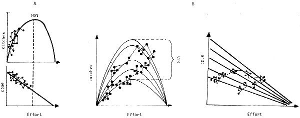
Fig. 14 A: Standard production model
B: Production model affected by a climatic variable
The points represent the theoretical course of a fishery.
Figure 14 B illustrates the fact that in this case the course is no longer necessarily reversible.
In the same way, it may no longer be considered that there is characteristic level of mortality by fishing F (criticial) for which the function R/rarr/S occupies the ultimate position at which the rate of replacement of the stock becomes insufficient and the stock collapses (Fig. 15A). It should, on the other hand, be admitted that the risk of collapse is always there, even for virgin stock, as is shown by observations on the California sardine in the past (Soutar and Isaacs, 1974) and the simulations of Laurec, Fonteneau and Champagnat (1980). A high risk zone could aslo be defined (hatched section in Fig. 15B) in which the fisheries administration could estimate that the bio-economic risk became insupportable.
It should be noted that, when catchability q varies according to the biomass (particularly if it increases when the biomass decreases), the replacement line R→S (Fig. 15B) will swing toward the left because of an increase in mortality by fishing F (not linked to an increase in the fishing effort) and will tend to approach the critical F zone, where risks of collapse are very high. These natural variations of the biomass, accompanied by variations of q, therefore involve important variations of the risk of collapse even if the fishing effort does not increase.
Moreover, the natural variations of q and therefore of F will also be reflected in variations of total catches, even in the absence of variations of the nominal effort because of the relation between F and catches recognized in the production model. In this case, there is confusion between the effects of the environment and those of fishing.
When the natural variations of recruitment are considerably superior to those produced by fishing and by changes in the size of the spawning stock, the stock-recruitment ratio could be very simply replaced by a model R = f (environment).
This model is usually considered as being unlikely to be affected by climatic variations, since it is not affected by recruitment variations. It has, however, been demonstrated that natural variations of abundance are accompanied by variations in growth, natural mortality, maturity, etc. It should therefore be admitted that this model will also be affected, which could lead to a revision of the rules as regards age at first catch, for example.
The recognition of the instability of an important natural resource immediately raises the problem of its continued monitoring, for example, by acoustic methods. It also raises the problem of prediction, since it then becomes fundamental to foresee in advance the evolution of the abundance so that the necessary management measures may be taken in time (prediction of R, of the biomass, of catches). Prediction models can be researched using relevant characteristics of the environment as predictive variables (cf. Garcia and LeReste, 1981; LeReste, 1982). They are, however, only useful if they really make possible a prediction sufficiently far in advance to enable industry and fisheries administration to react, and if the precision of the predictions is sufficient.
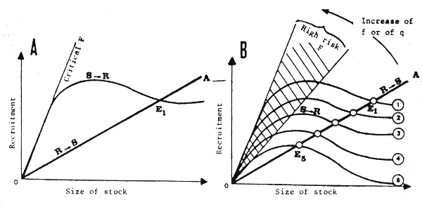
Fig. 15 Standard (A) stock recruitment relation and (B) affected by the environment
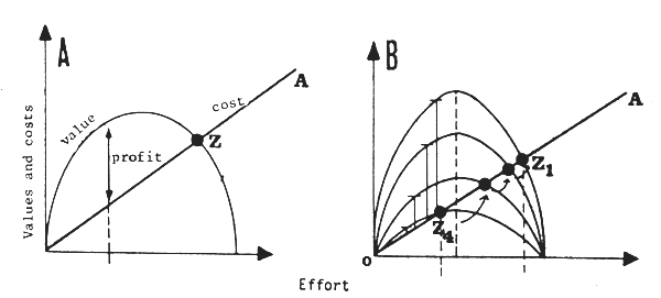
Fig.16 Standard (A) bio-economic model and (B) affected by the environment
The consequences described in Paragraph 3.1 concerning the production model can be expanded to the global economic model, widely used in fisheries economics. The standard model (Fig. 16A) assumes that there is an equilibrium point Z at which the development of the fishery will stop, and where the economic profit will be nil. The existence of natural variations in abundance involves the theoretical existence of a family of bio-economic models (Fig. 16B). There is therefore no longer a point but a line of equilibrium OA along which the fishery will tend to move when the stock passes from the abundance corresponding to the lower curve to that corresponding to the higher curve. The essential consequence is the existence of major fluctuations in profits (Fig. 17), and especially the possibility of exceptional increases, even in the case of overexploited fisheries. The natural fluctuations in abundance (and in particular the increases, regular or not, in the biomass) will therefore be powerful incentives for the exercise by professionals of very strong pressure on governments to obtain the aid necessary for expansion and reconversion (from the fresh fish market to meal, for example). They will finally be the source of overinvestment reaching astronomical levels, and out of all proportion to the levels of overinvestment that a more stable resource is able to generate in the context of a stable market.
![]()
![]()
![]()