


FIAP provides two main types of results: summary results, and the annual cash flows from which the summaries are derived. It can also calculate a number of other items, directly or indirectly. Some results can be viewed on graphs.
You can work with recalculation set to automatic, in which case FIAP is recalculated each time you enter anything; or you can work with it set to manual, in which case FIAP is only recalculated when you press the F9 function key or one of the Recalc buttons. The choice is made in the Options menu, where the option already selected is greyed Out and the remaining option (which you can change to) is shown in black.
If you work with recalculation set to automatic, recalculation proceeds in the background, which means that you don’t have to wait for it to finish before you enter more data. The advantage of working in the automatic mode is that everything is always updated as you work. However, if a lot of data is being entered it may be more comfortable to work in manual mode, because other figures will not be changing as you work, and it may feel more stable. When you are ready for results, you can force recalculation. With manual recalculation, you do have to wait until it is finished before entering more data.
![]()
The default is manual and there is an on-screen warning that recalculation is needed, which appears as soon as you change anything. This appears on the status bar at the base of the screen which will have the word Calculate to the right of Ready if recalculation is needed. You can force recalculation by pressing the P9 function key or one of the three other larger Recalc buttons provided for extra convenience in the What-if, Revenue-Expenditure and Results screens.
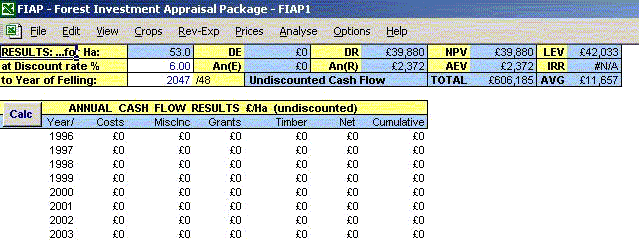
The 10 standard summary results available at all times are as follows. You have the option of calculating them per hectare or for the coupe as a whole (Options menu).
• DE |
Discounted Expenditure from now to any specified year |
• An(E) |
Annual Equivalent of DE for period specified |
• DR |
Discounted Revenue from now to any specified year |
• An(R) |
Annual Equivalent of DR for period specified |
• NPV |
Net Present Value (DR from now to any specified year |
• AEV |
Annual Equivalent of Net Present Value for period specified |
• LEV |
Land Expectation Value (NPV to infinity) |
• IRR |
Internal Rate of Return from now to any specified year |
• Cash |
Total net undiscounted cash from now to any specified year |
• Avg |
Average annual net cash for period specified |
At any time you can see these summary results by selecting GoTo from either the Edit or the View menus and choosing Summary Results. Whenever you go into the results screen FIAP automatically calculates the results to ensure that the results you are looking at are up to date. However, it is often more convenient to have them visible beside either the What-if screen or the Revenue-Expenditure model, especially during sensitivity analyses where the effect of changing individual parameters is being studied. See section 8.5.
The discount rate is shown at the top left of the summary results section. The default rate is 6.00%, but this can be altered to any desired rate; simply type in the preferred rate in whole number (i.e., 6 rather than 0.06, and don’t put a % sign after the number).
As a default, results are calculated from Year Now to the Year of Felling, whichever dates you enter for those years, but you can opt to measure the results for a shorter period of time if you wish. Under the discount rate is a cell in which you can enter any year you like between Year Now and Year Fell, and results will be calculated from now to that year instead of Year Fell. To reinstate the default, type =F into that cell.
To guard against the risk of forgetting that the year in that cell does not equal Year Fell, a warning appears in the cell to the left. If the projected year is less that Year Fell the warning reminds you that results do not include final felling, and if the projected year is later than Year Fell a warning also draws attention to the difference because although DE, DR, NPV and IRR are not likely to be affected, all the annual equivalents will be reduced. (LEV is not calculated at all if this year is not equal to the year of felling.)
DE and DR are, respectively, the sum of all expenditure and income items from Year Now to Year Fell (or less if the above option is in force), each discounted at the specified discount rate for the appropriate number of years. DR includes receipts from timber, miscellaneous sales and grants. An(E) and An(R) are the equivalent annual payments and receipts, calculated for the same time period and discount rate.
NPV is DR-DE. It has often been known in forestry as Net Discounted Revenue (NDR), but NPV is the more widely accepted term. AEV is the annual equivalent net payment or receipt for the same period and discount rate; it is equivalent to An(R)-An(E).
LEV is NPV to infinity, but not including the cost of land. LEV is derived from NPV, using the same discount rate and time period, but there are four conditions in which this measure is not calculated, and #NA is shown even when NPV has a value. As it is designed largely to indicate the price which could be profitably paid for land, it is not calculated if a price for land has already been entered in the land cost box. As it measures all future profits (or losses) it cannot be calculated unless the discount rate is more than zero. It is not meaningful unless the final felling is included, and unless the period of NPV is no longer than final felling (because of the relationship with AEV explained below). Finally, nor can LEV be meaningful when crop components have different planting years. Even when all planting years are the same, with multiple crop components this measure should be treated with caution. When LEV is shown, its annual equivalent is given by AEV, which can then be understood as a perpetuity (an infinite annuity), as well as an annuity running from now to the year of felling.
Normally NPV tends to be high with low discount rates and to decline rapidly as the discount rate is raised. At some point it becomes negative, and IRR is the discount rate at which NPV equals zero. The IRR function in the summary results is designed to return the IRR at rates of up to about 100%. At rates as high as that IRR is quite meaningless in forestry; and if circumstances are not normal, alternative means of finding IRR may have to be used.
Rates of IRR can be raised to a very high level when early costs are almost offset by grants, as can often happen in private forestry. If the costs are completely offset (which is not unknown), there may be no rate of discount at which NPV=0, and therefore no IRR. Under some circumstances - e.g. when early costs are soon covered by grants, but then later the cash flow becomes negative again because of high maintenance charges, before turning positive with thinnings and fellings - NPV can be reduced to zero by more than one rate, and there are therefore multiple IRRs (impossible though that may sound).
If there is no IRR below about 100%, IRR returns #NA (for not available). In the event of there being multiple rates, it will probably give the lowest rate is comes to, though it might return #NA, depending on cash flow circumstances. For this reason an IRR test was developed.
To cope with any uncertainty about multiple rates of IRR, an IRR test has been provided which can be found under the Analyse menu or the GoTo under either the Edit or View menus. It is simply a column of NPVs calculated at integer rates of discount from zero to 100%. You can scan down that column looking for changes of sign. No change of sign means there is no IRR (or, if there is one, it is above 100%; and being so high makes it pretty meaningless) A single change of sign shows roughly where the IRR is; multiple changes of sign indicates multiple rates of IRR. It is possible to view this column on a graph: select the Graph Results then IRR Test command from the Analyse menu.
When such difficulties are encountered with IRR there would have to be very strong reasons indeed for using it as a criterion of profit in preference to NPV - strong enough to motivate the operator to find out from technical economic literature how to resolve the problems.
The final two summary results are undiscounted cash figures for the specified range of years total net cash for the duration specified, and the annual average over that period These figures may be useful for farmers and other private investors considering forestry, who want to know their projected cash flow commitments, but who may prefer to apply their own intuitive discount rate Such investors may also find the annual cash flow figures of interest.
The second standard set of results which are always available are the annual cash flows. These are the data from which FIAP calculates the summary results. They are not discounted and are always shown per hectare (i.e., they are not scaled up when the summary results are shown for the whole coupe). There are six columns of data (alongside the years starting .with YearNow), as follows, which are explained in the paragraphs below.
• Costs |
• Timber |
• Miscellaneous income |
• Net cash flow |
• Grants |
• Cumulative cash flow |
These three columns are derived from the three sections of the Revenue-Expenditure model. Single costs or receipts are allocated to the year in which they occur, and annuities are allocated to each of the years in which they occur. Each year includes all financial items incurred in that year, plus the annual overhead charge per hectare, if any.
These receipts are calculated separately for each crop component in the money yield tables, where the prices and volumes are multiplied together. Each year includes all the thinnings in any productive component predicted for that year, and felling income is added in the year of felling. The figures take account of settings in the What-if screen, and are corrected by the appropriate inflation factor and weighted according to the relative size of the various components.
The net cash flow for each year is simply the sum of timber income, miscellaneous income and grants, less costs. It is possible to view these results on a bar chart: select the command Graph Results then Net Annual Cash Flow from the Analyse menu.
The cumulative cash for any year is simply the sum of the net cash flow up to that point. It gives a useful indication of the total fortunes of the investment so far. This column of figures can also be shown on a graph (Graph Results then Cumulative Annual Cash Flows from the Analyse menu). When the level is falling the crop is costing money; when it is rising income exceeds costs; and when there is no change in level from one year to the next, the two balance each other.
An important factor in investment appraisal is the felling year at which DR (discounted revenue) is maximised. This result is rather different from the others because it is not a final answer, but one likely to be used in reaching a set of results You could find this by trial and error, altering the Felling Year iteratively until you found the rotation which gave the highest DR. And indeed you could do this for any measure of performance (e g, NPV or IRR) instead of DR.
The iterative procedure is quite accurate, but the process may be automated (for DR) by using the Calculate Max DR command in the Analyse menu which works out DR figures for a range of felling years in one move. When you select this command you are prompted for the earliest and the latest likely felling years: DRs are calculated for that range of years, and placed in a column against the range of years you have selected.
FIAP will also find the year in which DR is maximised, and offer you the option of recording it in the Year of Max DR on the What-if screen. If you select OK, you will be offered the further choice of recalculating the sheet using that year as the year of felling.
This procedure is quite slow, even with a fast machine, and it speeds things to specify a narrow band of years. However, the band has to be wide enough to span the maximum DR. If the maximum DR is either the lowest or the highest year, then the optimum year has not been safely identified, and the exercise must be repeated with an amended range of years.
The results can be viewed on a graph which makes it easier to check whether the maximum has been found. Select the Graph Results then Maximum DR from the Analyse menu.
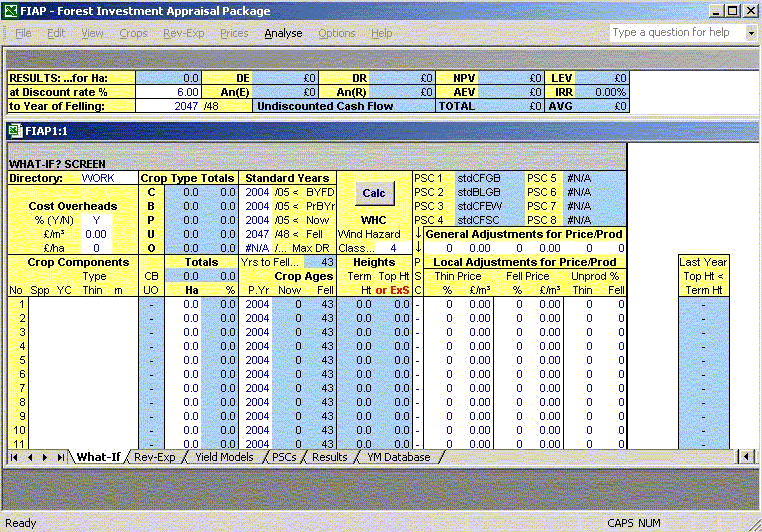
The first two commands in the Analyse menu assist your analysis by splitting the screen window into two panes, with the summary results in the tope and the What-if or the Revenue - Expenditure screen in the lower one. Due to the limitations of the spreadsheet package, rather than FIAP, it is not possible to alter all the variables. You will notice that in the menu, only Analyse is not greyed out, and from this you will notice that Reset is the only option available. This means it is not possible to load in new yield models for new crop components, nor can you load in new PSCs. However you are able to change areas, years, discount rates, WHC, cost overheads, price and production adjustments and PSCs (as long as it is to one already loaded).
You can make allowed alterations as often as you like. It is probably best to have recalculation switch to automatic mode.
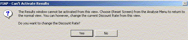
The only variable you can change in the top pane is the discount rate. Clicking on the top pane will produce a warning box asking if you wish to change the discount rate.
Remove the screen split with the Reset Screen command in the Analyse menu.
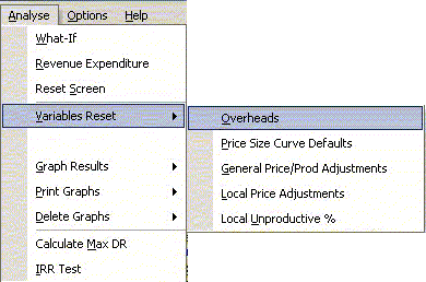
You can always reset any of the variables one by one, but commands are provided in the Analyse menu to speed up the task by resetting batches of variables. There are five groups of figures to rest, accessed by the Variables Reset command.
This command resets the three overhead settings in the What-if? screen, Y for percentages and zero for the other two. It does not alter the percentage figures entered against each cost in the Revenue-Expenditure model.
If you overwrite the automatic PSC selection (1 or 2) to use other price-size curves, you may later wish to reinstate the default. This command resets all 20 crop components.
This command resets all six of the general price and productivity adjusters to zero.
This command resets all the local price adjusters to zero.
This command resets all the local productivity adjusters to zero.
FIAP allows you to express five sets of results on graphs, accessed by the Graph Results command in the Analyse menu. With all but the Max DR calculation, you can leave graphs in place as you alter the figures in FIAP, and they will alter in response to new data. If recalculation is set to auto, this will happen each time you enter a figure; if recalculation is set to manual it will happen each time you recalculate the sheet. When you no longer want them, delete the charts with the Delete Graphs command or by clicking on them with the mouse and pressing delete on the keyboard.
FIAP divides all crop components into four types: productive conifer (C), productive broadleaves (B), unproductive planted areas (U) and open space (0) (see section 4.2). Figures for the area and percentage proportions of these four types is shown at the top of the What-if screen, but it may be helpful to see this on a pie chart, which is possible f at least two types of crop have been entered.
When you select this command the column of net yearly cash flow figures are shown on a bar chart, with net costs below the X-axis, and net receipts above.
When you select this command the column of cumulative yearly cash flow figures are shown on a bar chart. In periods of cost the level decreases; in times of receipt they rise; and no change from one year to the next indicates that receipts balance costs.
Having calculated DRs for a range of years, it may be very helpful to be able to see the results on a graph. It stands out immediately whether the optimum felling year has been covered, and how great the financial sacrifice may be of felling before or after the optimum. It has to be stressed that what is being considered is the optimum for the coupe as a whole, not individual crop components.
This graph performs three functions. You can view the NPV for any specified range of discount rates (between 0% and 100%) as a quick check on the sensitivity of NPV to changes in the discount rate. Second, if the range you select spans the point where NPV become negative, you can see the approximate IRR where the curve crosses the zero NPV line. And third, if you are checking for multiple rates of IRR or none, you can graph the full range of rates. The graph is not then very large scale, but it provides a visual indication of the areas of the IRR Test column to inspect more closely, as described in the paragraphs on IRR in Section 9.2.
This command in the Analyse menu allows you to choose which of the five graphs to delete. If you select a graph which is not drawn, FIAP will ignore the command.
You can print off the graphs you have created with the Print Graphs command in the analyse menu. It offers you a choice box from which to select the graph you wish to print. You can print whatever you like with the Print User command in the File menu (see section 10). If you select a graph which is not drawn, FIAP will ignore the command.
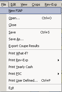
Printing commands are provided in the File menu, as summarised below.
The Print What-if command will include the summary results at the foot of the What-if screen on a single page.
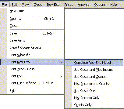
The Print Rev-Exp command offers you a choice of which parts of the Revenue-Expenditure model to print, because if parts of it have not been used you may not want to print it all. The final option allows you to make your own selection. This command is also available from within the Rev-Exp menu.
The Print Yearly Cash command will print the annual cash flows, on several pages if necessary. Where it flows onto two or more pages, the titles of the columns are repeated on second and subsequent pages.
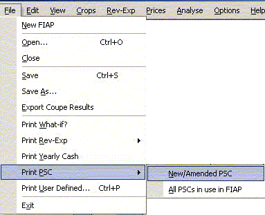
The Print PSCs command offers you a choice of printing only the new or amended PSC, or all those currently in use in FIAP. This command is also available from within the Prices menu.
The Print User command allows you to make your own selection of what to print.
You can change one or more parameters and recalculate to see the effects. By calculating results successively for two carefully selected sets of parameters, the financial implications of various kinds of change can be measured, e.g., felling before or after the financially optimum year, changing the proportions of the crop components, or changing the species themselves within those components. FIAP can calculate results for fresh assumptions very quickly, but it does not actually compute the differences directly.
Similarly, by calculating totals for a succession of coupes, using the same discount rate and base year for discounting, and adopting consistent assumption throughout, aggregate results for a collection of coupes can be built up. Once again, FIAP can calculate such results quickly (though keying in the data may take much longer) and it can provide aggregation directly using the Coupesum extension.
Within the File menu there is an option Export Coupe Results. This transfers the following data to a separate file called the Coupesum.
This has the added benefit of talking up much less space on your computer than saving the entire FIAP model. It also provides totals along the bottom row.
You can access your results by coming out of FIAP (either by quitting or toggling between Program Manager and FIAP – an easy way to do this is by holding down the ALT key and pressing TAB) and going into Coupesum.
This takes you into a spreadsheet containing a single screen entitled Coupe Summary Analysis. In order to add coupe results they must have the same standard details. For example if one coupes results were calculated at a discount rate of 6% they cannot be compared with another coupe with a discount rate of 8%. A warning message appears if results are not compatible.
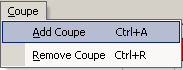
The first coupe you enter sets the standard details for that particular analysis until you start again by either removing all the results from the screen by using the Remove Coupe command from the Coupe menu or by using the New command from the File menu. You cannot remove the top coupe by this method unless it is the only one in the table. Another method is to use the mouse and the Delete button on the keyboard.
The Open command under the File menu allows you to retrieve saved and complete summaries. Summary results have the suffix .sum. The Save and Save As commands allow you to save the current summary. Coupe results have the suffix .cpe. The Print command prints it out.
Within your summary you can add or remove results by using the Add Coupe and Remove Coupe commands respectively from the Coupe menu. The table can be as long as is required and is never less than eight rows.
