Methods

Field method
Analytical technique

The National Goat Breed Survey was carried out by three consecutive graduate students from Alemaya University of Agriculture between January 1990 and June 1993. A standard survey method was followed by each student to ensure comparable data. Each student's data set was analysed independently after completion of the field survey. When the final student completed-his survey the three data sets were amalgamated and analysed as one.

Field method

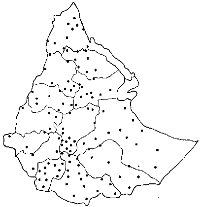
Each region surveyed was stratified by altitude and ethnic group. Peasant Associations (PAs), the smallest administrative unit in Ethiopia and Eritrea, were taken as sampling sites. Sites were selected at 500 m intervals along altitude transects spanning the known ethnic range (Figure 2). The survey included only one visit to a sampling site at which whole flocks of goats were sampled until about 500 goats had been physically measured.

A total of 21 variables were selected from the FAO (1986) goat breed descriptor list. These were divided into morphological and other variables. The morphological variables were further divided into qualitative and quantitative:

· Qualitative: sex, dentition, presence of beard, presence of ruff, presence of wattles, head profile, coat pattern, coat type, ear form, horn shape, horn orientation.

· Quantitative: body length, chest girth, height at withers, pelvic width, ear length, horn length, body weight.

The other variables included:

· Parturition history of does as recalled by owner: total number of parturitions, single births, multiple births.

· Source of animal: whether home-bred, purchased, given etc.

Although it is customary to describe breeds in terms of mature females, whole flocks were sampled to obtain information on the size of flock owned and flock structure.

The dentition classes used in the survey were not entirely uniform between students. In order to standardise the classes for the overall analysis, the more refined classes were amalgamated into the broader categories of milk teeth, one, two, three and four pairs of permanent incisors. Goats were measured using a plastic tape measure and weighed using a 100 kg × 500 g spring balance suspended from a metal tripod. Weights were recorded to the nearest half kilogram. Flocks were sampled early in the morning before grazing. To facilitate the survey local Ministry of Agriculture veterinary personnel accompanied the survey team to vaccinate or treat the goats brought to be measured.

Information, reported by goat owners, on the reproductive performance of each doe sampled was recorded. Data on parturition history, number and types of birth enabled the estimation of the average litter size and the average reproductive performance.

A questionnaire was used to collect information on housing, feeding, breeding management, product use and the traditional use of goats at each site.

Figure 2. Map of sampling sites by ecological zone.

The main field problems encountered affecting the data were the reluctance of some goat owners to bring their very young kids to be surveyed. This led to slightly distorted flock structures for the Worre, Barka and Nubian goats.

Analytical technique

The analytical goal was to determine the morphological resemblance or dissimilarities within an assemblage of animals. If there are initial classes such as uniform animal populations indicating a breed type, or commonly accepted, but not established, local names of breed types, and if the total sample population can be classified into these categories, discriminant analysis can be used to justify group differences (Klecka 1980). In the absence of distinct initial classes, the animal population may be assumed to be a heterogenous set divisible into more homogenous taxonomic groups which may represent breed types or varieties (Aldenderfer and Blashfield 1984). Multivariate analysis techniques are usually used to explore the factors of dissimilarity within a population, and eventually reorganise a heterogenous set of observation units into relatively more homogenous groups from the total population.

For this study the unit of analysis was the population of mature female goats at each site characterised by the mean of the continuous variables and the frequency of discrete variables. Mature females were selected because it is customary to describe a breed by a description of the females because they usually exist in larger numbers and it is easier to determine their stage of maturity than for males. The variables selected to describe the mature female goats included continuous variables, such as height at withers or ear length, and discrete variables such as coat colour or ear orientation. Variables were screened for variability and discriminating power. A total of 35 variables were finally selected.

The number of animals measured at each site depended upon the precision required and the variability in the population. Coefficients of variation on growth traits have been observed to be up to 35% (Peters 1985). For significance at the 5% level, 100-300 mature females are required per site (Bruns 1992), implying a target sample size of 500 goats from any site. A total of 103 sites were included in the analysis. Thirteen additional sites were considered as supplementary observations due to the small number of animals recorded, implying high variability for means and frequencies.

Variation trends: Principal components analysis

In order to identify the most important multifactorial variation trends across the populations the 35 variables, naturally correlated, were transformed into as many independent principal components using the procedure ANCOMP of ADADSAS software (ADDAD 1990).

Appendix II presents the correlation of the variables with the first seven principal components. The first three principal components account for 45% of the total variance of the model. They indicate the major contrasts between the goat populations.

The first principal component contrasts goat populations with:

High positive value on Axis 1	High negative value on Axis 1
- Ear length	- Curved horn shape
- Height at withers	- Lateral horn orientation
- Straight horn shape	- Plain coat colour pattern
- Brown coat colour	- Smooth and short hair
- Patchy coat colour pattern
- Ruff with hair on the thighs

The second principal component segregates:

High positive value on Axis 2
- Ear length
- Chest girth
- Body weight
- Weight to height at withers ratio
- Ear to height at withers ratio
- Lateral horn orientation

The third principal component is a contrast of:

High positive value on Axis 3	High negative value on Axis 3
- Height at withers ratio	- Horn to height at withers
	- Long hair

The fourth principal component compares goat populations with:

High positive value on Axis 4	High negative value on Axis 4
- Height at withers	- Upward horn orientation
- Backward horn orientation	- Beard
	- Black coat colour
	- Grey coat colour

Classification: Cluster analysis

The first 15 principal components, accounting for 94% of the total variance, were considered to develop the classification by cluster analysis. The set of 103 observations against those principal components was clustered by a single-linkage, agglomerative, hierarchical and non-overlapping (SAHN) technique which is the most widely applied method of clustering in biological systematics (Sneath and Sokal 1973; Aldenderfer and Blashfield 1984). The Mahalanobis distance was the similarity coefficient used to develop the classification tree from which the desired number of clusters was obtained. The procedure of ADSAS was used.

The classification tree or dendogram (Figure 3) allows the exploration of the general pattern of relationships between the observation units. Heuristic decisions were taken to determine the number of clusters. The choice was largely subjective but efforts were made to find one with the most meaningful biological interpretation. The initial results of the cluster analysis were mapped for consistency. Population means and frequency were computed for the newly assembled populations. A few (nine) misclassified sites, forming one cluster, were reclassified into the other 14 clusters. The geographical representation of that reclassification was pertinent.

Figure 3. Hierarchical classification tree.

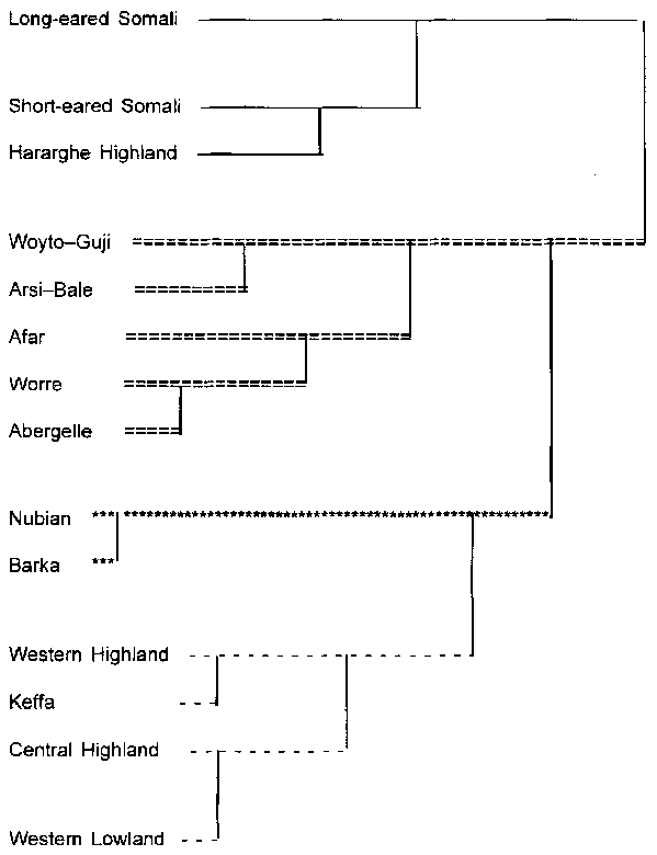
The dendogram shows four distinct groups (families) of goat populations. Figure 4 represents the projection of the inerty clouds of those four major clusters in the coordinate system defined by Axes 1 and 2 of the Principal Component Analysis.

A 14-cluster solution was found to be meaningful (Table 3).

Naming livestock types can be a contentious issue. In Africa breeds are often named after the main ethnic group keeping them, e.g. the Boran cattle breed, the Boer goat etc. However, some of these names date from the colonial era and can take on a pejorative meaning when used in modern times, e.g. the Galla goat in Kenya. The breeds can also be named after the region in which they are found, which is sometimes synonymous with ethnicity. Types can also be referred to in a more neutral manner by naming them after an important identifying characteristic, e.g. West Africa Dwarf goat, the Long-eared Somali goat. The names given to the clusters (Table 3) reflect geographical location as much as possible rather than ethnic group.

Figure 5 describes the distribution of the goat types in Ethiopia and Eritrea and Table 4 presents estimates of the population of each goat type.

Figure 4. Inerty clouds of four major clusters in co-ordinate system PC1-PC2.

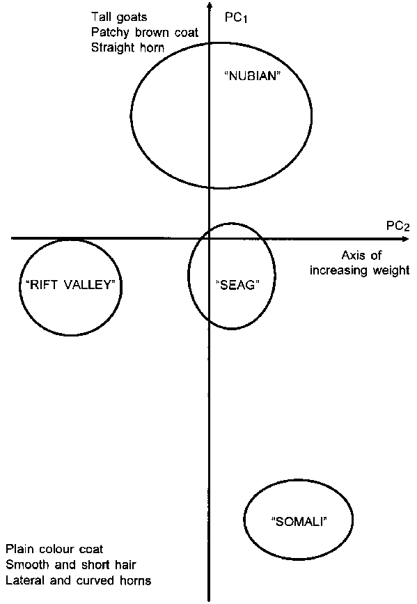
Table 3. The goat types of Ethiopia and Eritrea.

Cluster number	Name
1	Nubian
2	Woyto-Guji
3	Arsi-Bale
4	Central Highland
5	Afar
6	Western Highland
7	Keffa
8	Barka
9	Worre
10	Abergelle
11	Short-eared Somali
12	Hararghe Highland
13	Long-eared Somali
14	Western Lowland

Figure 5. Geographic distribution of goat types.

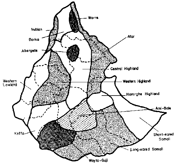
Table 4. Distribution and estimated population of goat types.

Goat type	Distribution	Population
Nubian	Lowlands of western Eritrea (Gash and Setit)	200,000
Barka	Lowlands of western Eritrea (Gash, Setit and Akordat)	600,000
Worre	Highlands of northern Eritrea (Keren and Sahil)	500,000
Afar	Rift Valley areas of Eritrea and north-eastern Ethiopia (Afar region)	1,000,000
Abergelle	Mid-altitude of southern Tigray and northern Wollo, along Tekeze valley	300,000
Central Highland	Highlands of southern Eritrea (Akale Guzay and Seraye) and northern Ethiopia (Tigray, Wollo, north Gondar and north Shewa)	6,000,000
Western Highland	Highlands of western Ethiopia (south Gondar, Gojam, eastern Wellega and Illubabor)	3,000,000
Western Lowland	Lowlands of western Ethiopia (Metekel, Asossa and Gambela)	400,000
Keffa	Keffa, part of Illubabor and south Shewa	1,000,000
Arsi-Bale	Highlands of Arsi, Bale and south Shewa	600,000
Woyto-Guji	Gamu-Gofa and eastern Sidamo (Guji)	900,000
Hararghe Highland	Highlands of eastern and western Hararghe	1,000,000
Short-eared Somali	Lowlands of Ogaden	1,500,000
Long-eared Somali	Lowlands of southern Ogaden	1,500,000