

Understanding how land degradation affects food production is critical to global food security. However, assessing the causal linkages in this relationship can be a complex process: evidence is often contradictory, with studies reporting effects that range from negligible to severe.26, 27 References to positive correlations between high yields and land degradation can even be misinterpreted as a causal relationship.28 Isolating the direct impact of land degradation on agricultural productivity can also be challenging due to numerous confounding factors including the interplay between environmental and management practices. This report presents new global evidence on the causal relationship between cropland degradation and yield loss. It explores the underlying pathways that contribute to this relationship – pathways that may need to be avoided in the future to effectively address land degradation and achieve food security goals.
While land degradation occurs across all types of agricultural land, findings related to croplands provide important information on how to ensure sustainable food production and reduce pressure on natural ecosystems – both of which are fundamental to achieving food security. Croplands account for nearly one-third of all agricultural land, and form the basis of food provisioning and of regulating and cultural services.29, 30 Accordingly, croplands produce the vast majority of global kilocalories and proteins. Cereals alone contribute about 43 percent of global caloric intake, with vegetables, fruits, and roots and tubers adding another 15 percent, and sugar crops providing an additional 8 percent.31 Additionally, one-third of all croplands are used to grow animal feed, indirectly contributing to protein availability in addition to the plant-based proteins directly consumed by humans.
Cropland expansion has accelerated in the twenty-first century, significantly affecting forest loss, wildland fragmentation and pasture conversion – a trend in direct conflict with SDG 15.32 The contribution of these biomes to food security complements the central role of cultivated crops in nutrition, particularly for forest-dependent and pastoralist communities.33–35 Furthermore, on average every year nearly 4 Mha of cropland are being abandoned, possibly due to degradation, leading to losses in production.36 Addressing degradation in croplands, and its implications for yield gaps and land abandonment, would therefore relieve pressures on other types of land cover.
For land that is currently in production, yield gaps are key to understanding the impact of land degradation on crop production (see Chapter 1). They represent the difference between the maximum attainable yield for a given crop in a specific environment and the actual yields achieved by farmers. Figure 8 shows the global distribution of agroecological yield gaps for 2020, drawing on FAO’s latest Global Agro-ecological Zoning (GAEZ v5).37 These agroecological yield gaps measure the difference between actual yields and attainable yields based primarily on environmental conditions for ten major crops: barley, cassava, maize, oil palm, rapeseed, rice, sorghum, soybean, sugar cane and wheat. Together, these crops account for over 80 percent of all harvested food energy and more than 60 percent of global harvested area.38 The data underlying the figure are in broad agreement with statistical yield gaps, which use attainable yields from the best-performing farmers under real-world conditions and account for additional socioeconomic and institutional constraints.39
Figure 8 Agroecological yield gaps for ten major crops, 2020
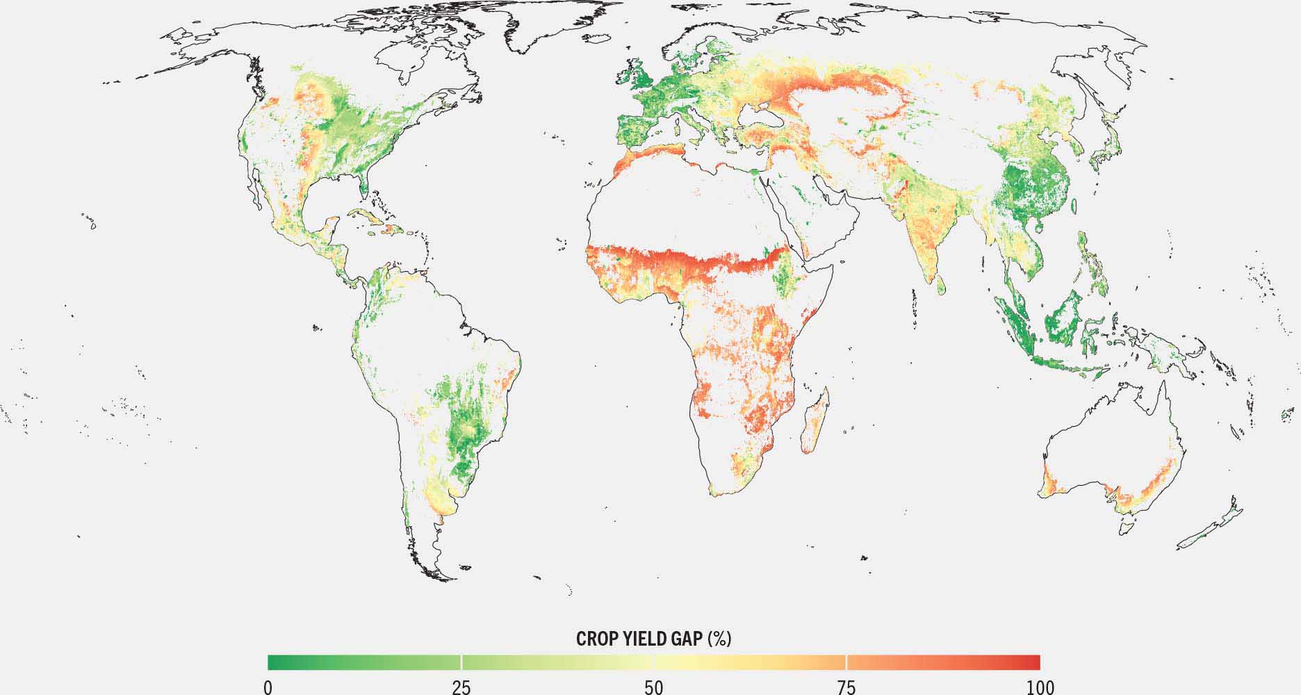
SOURCE: Hadi, H. & Wuepper, D. 2025. A global yield gap assessment to link land degradation to socioeconomic risks – Background paper for The State of Food and Agriculture 2025. FAO Agricultural Development Economics Working Paper 25-16. Rome, FAO.
To inform effective policies, it is essential to distinguish between: 1) all-cause yield gaps (ACYG) – which reflects the combined effects of diverse biophysical, management and socioeconomic constraints; and 2) more specific degradation-induced yield losses (DIYL) – which refer to the portion of yield gap directly attributable to land degradation due to human activity. While isolating the precise contribution of degradation to ACYG is analytically complex, examining its magnitude and spatial patterns in relation to indicators of land degradation can provide insights into how much agricultural potential is being lost. However, establishing a causal link between land degradation and yield gaps is highly challenging, due to the gradual, cumulative and context-specific nature of degradation processes.
If land degradation indicators and ACYG are mapped together, the results show that yields are higher (and hence yield gaps smaller) in areas with higher land degradation. This is because cropland degradation is strongly correlated with intensive agriculture.40 However, land degradation is only one of many factors that can impact yields. To isolate the impact of land degradation on yield gaps, it is necessary to control for the impacts of other factors, including management choices (input use), agroecological conditions (soil type, climate, topography), and socioeconomic and institutional characteristics.
The use of a debt-based approach to measure land degradation helps to capture and isolate the impacts of human activity on land degradation indicators (Box 7). This approach has revealed that, compared to native/natural conditions, global tree cover had fallen by 30 percent, carbon stored in biomass had decreased by 20 percent (average for above- and below-ground carbon) and soil erosion had increased almost fourfold due to human activity, as of 2010.23 The consequences of these changes for global food security take the form of increasing yield gaps, where a 10 percent increase in land degradation debt is associated with an approximately 2 percent increase in average statistical yield gaps for circa 2010.40
Box 7Debt-based approach to assessing human-induced land degradation
Land degradation debt can be defined as the difference between the current values of specific indicators – soil organic carbon (SOC), soil erosion and soil water – and their values without human activity. The process used to model the counterfactual values applies recent advances in remote sensing, machine learning and computational resources, to separate human-induced change from natural degradation processes.23 This is achieved by modelling each degradation indicator to proxy baseline conditions using the following historical benchmarks:
- Soil organic carbon: native SOC.41
- Soil erosion: land cover in protected areas.42
- Soil water: long differences based on the European Space Agency Climate Change Initiative’s Soil Moisture dataset.43–45
Regardless of the differences in historical benchmark, each debt measure captures the effects of human activity on agricultural land compared to native/natural conditions. These data are fed into a machine-learning model that incorporates environmental drivers of change to isolate the native/natural state of land in the absence of human interference. The counterfactual soil organic carbon is modelled under a prehistoric “no land use” scenario representing pre-agricultural conditions (~10000 BCE), while other environmental drivers of soil organic carbon remain unchanged.41 These values are then compared against estimates of current soil organic carbon taken from the FAO Global Soil Organic Carbon Map (GSOC Map),46 to quantify human-induced losses of soil organic carbon, or SOC debt.
For soil erosion, a machine-learning model is similarly trained using data from protected areas, where land cover is assumed to be relatively unaffected by human activity, thus approximating vegetation cover in historical times. See the rationale and limitations of this common approach in Hengl et al. (2018).47 The model learns how native land cover relates to environmental predictors (e.g. temperature, rainfall). It then applies this relationship to all regions to estimate what the land cover would be in the absence of human land use. This estimated counterfactual land cover is used as the main input in the soil erosion model (with all other soil erosion drivers held constant) to simulate natural erosion rates without human-induced changes. These are then compared with current soil erosion rates42 to quantify human-induced erosion, or soil erosion debt. Further details can be found in Wuepper et al. (2021).23 The maps in the figure illustrate two examples of this method showing the components of the SOC and soil erosion debt calculations for Ethiopia and the United States of America.
Importantly, this approach does not assume that historical land conditions were optimal for agriculture. Rather, using a historical benchmark provides a reference point to track changes over time and evaluate the long-term impact of human-induced land degradation on current crop yields. This enhances comparability across regions and facilitates the assessment of restoration opportunities. Furthermore, land degradation is treated as a continuous variable, eliminating issues associated with arbitrary thresholds.48
FIGURE COUNTERFACTUAL AND CURRENT LEVELS OF SOIL ORGANIC CARBON AND SOIL EROSION RATE: ETHIOPIA AND THE UNITED STATES OF AMERICA
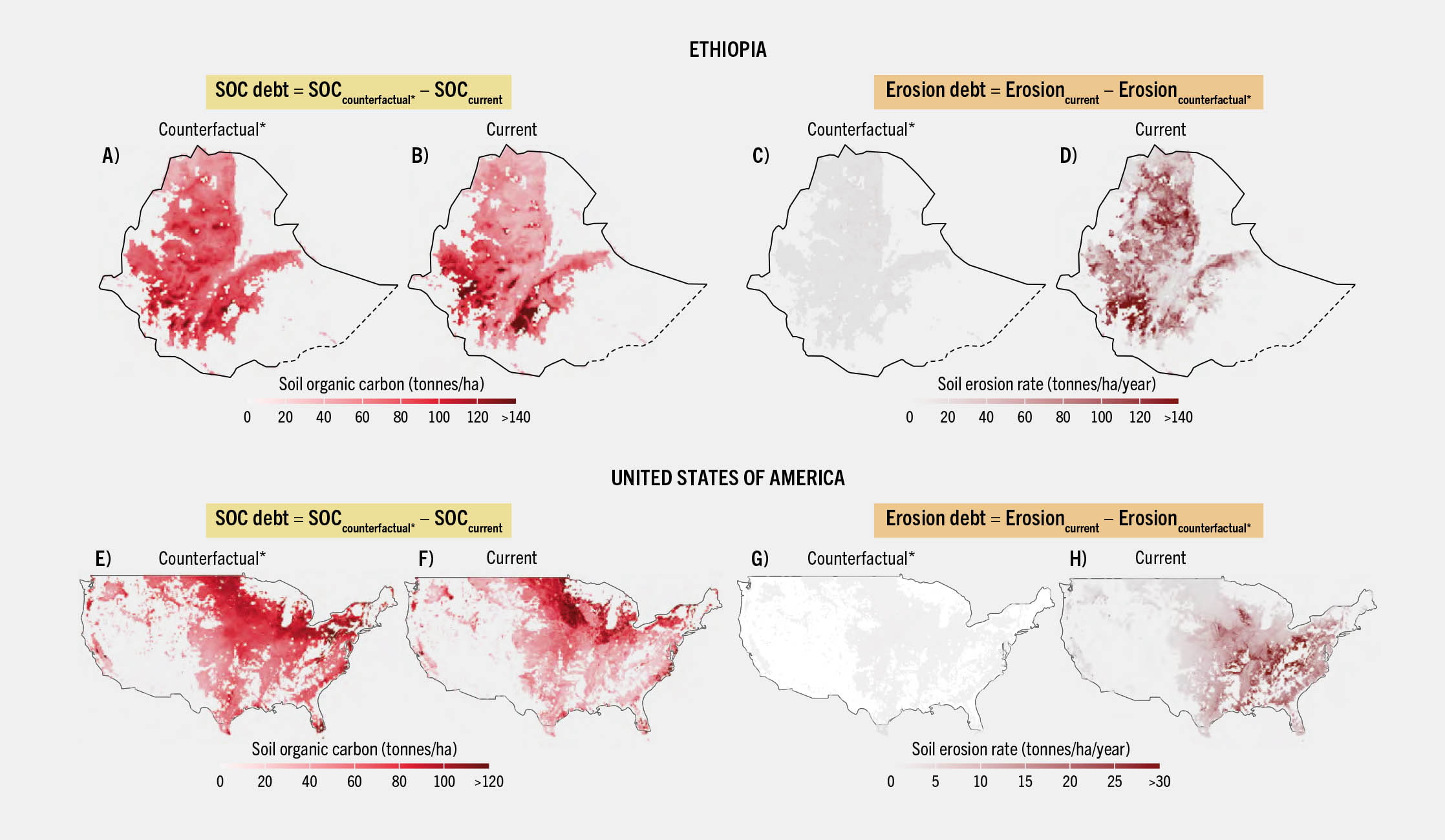
SOURCE: Hadi, H. & Wuepper, D. 2025. A global yield gap assessment to link land degradation to socioeconomic risks – Background paper for The State of Food and Agriculture 2025. FAO Agricultural Development Economics Working Paper 25-16. Rome, FAO.
Estimating the extent of DIYL on croplands relies on a wide range of global databases and state-of-the art analysis methods. By accounting for input intensities, as well as many other factors that affect yield gaps, this approach isolates the true biophysical yield penalty caused by land degradation, which is often masked when inputs fully or partially compensate for its effects. Box 8 provides further detail on this methodology.
Box 8Estimating the causal links between human-induced land degradation and yield gap at the global level
The causal relationship between land degradation and yield gap, referred to here as degradation-induced yield losses (DIYL), is analysed using cross-sectional geospatial data and a control-on-observables regression approach. A global dataset at 10-km resolution is employed, consistent with yield gap measurements. The empirical method employed follows Hadi et al. (2025).40
A causal forest model – a modern causal machine-learning method49, 50 gaining traction in applied economics51–53 – is applied to estimate how yield gap changes with land degradation in each grid of the latest global cropland map. The model is set up to quantify the percentage change in yield gap per 1 percent increase in land degradation indicators defined in Box 7, allowing for assessment of the total impact of soil organic carbon debt, soil erosion debt and soil water debt on current yield gaps.
To help ensure that the estimates are robust, the model controls for a wide range of factors (see Table A1 in Hadi and Wuepper [2025]).39 These include the following:
- Natural and environmental variables: climate conditions (e.g. temperature, precipitation, solar radiation), soil properties and topography.
- Agricultural management features: fertilizer and pesticide use, irrigation, farm machinery and agricultural employment.
- Socioeconomic and institutional factors: gross domestic product, human development index, road density, travel time to cities, access to electricity, mobile phone subscriptions, property rights protection, environmental policy stringency and enforcement, and corruption perception.
The magnitude of the estimated impacts of land degradation on yield gap (i.e. DIYL) is then overlayed with gridded data on socioeconomic factors (e.g. population, poverty, stunting), to identify vulnerability hotspots.
The approach demonstrated here improves upon previous methods54–56 for measuring land degradation, with a focus on croplands. Earlier studies identified degraded land based on observed negative trends in satellite-measured vegetation indices or net primary productivity over recent decades, accounting for only a limited set of confounding factors (e.g. rainfall, fertilizer use). Others relied on criteria such as slope, soil quality (using only soil water as a proxy) and rainfall. In contrast, the present model identifies degraded land using a more comprehensive and direct representation of degradation processes on croplands and, thanks to the causal forest model, isolates the impacts on latest yield gaps.
FIGURE CONCEPTUAL FRAMEWORK FOR ESTIMATING DEGRADATION-INDUCED YIELD LOSSES
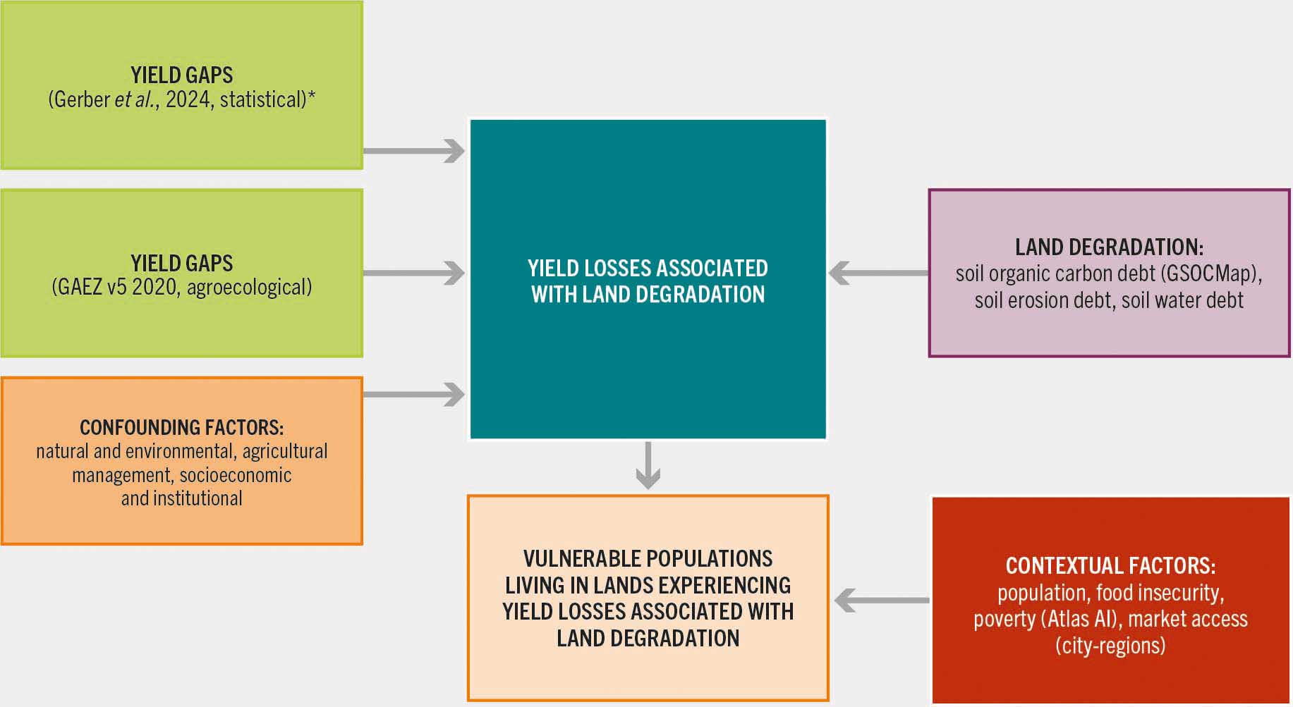
SOURCE: Hadi, H. & Wuepper, D. 2025. A global yield gap assessment to link land degradation to socioeconomic risks – Background paper for The State of Food and Agriculture 2025. FAO Agricultural Development Economics Working Paper 25-16. Rome, FAO.
The identification of the causal links between land degradation and yield gaps allows for the estimation of the extent to which yield gaps have already widened specifically due to degradation, as well as facilitating the identification of areas where they are mainly driven by other factors. Crucially, this analysis also facilitates the assessment of socioeconomic vulnerability hotspots, thus linking SDG Target 15.3 more directly to food security outcomes under SDG 2, as well as to poverty (SDG 1) and livelihoods (SDG 8).
Costs of land degradation: global losses in provisioning services from croplands
The global cost of land degradation has been quantified by a number of studies, and it varies significantly according to the ecosystem services and biomes being assessed.30 It depends on the baseline used, as well as on how ecosystem and provisioning services are valued. Including all costs of land degradation – from those due to decreased production borne by private land users, to those arising from lost ecosystem and cultural services borne by society at large – a global study found that the annual cost of land degradation is about USD 300 billion. More than three-quarters of these costs are attributed to land use and land cover change (LUCC), and the majority of the costs globally are borne by the public rather than by private land users.30 While this observation makes addressing land degradation partially a public good, understanding the incentives of land users is critical to facilitate action to address degradation for both private and public benefits.
The extent to which land degradation affects crop production, yield gaps and land abandonment has direct implications for the availability dimension of global food security. For hundreds of millions of farms that depend on crop production, it also has an important impact on livelihoods. This section, therefore, focuses on the costs arising from losses in cropland provisioning services; it uses the model described in Box 8 to assess the causal land degradation–yield loss relationship. This chapter later examines the prevalence of land abandonment in cropland areas to understand yield loss in relation to land that was in production at an earlier point in time.
Reduced yields decrease overall crop production, and hence the availability of dietary energy, potentially exacerbating undernutrition in vulnerable populations. Additionally, these losses have direct economic implications, as reduced agricultural output leads to declining revenues for farmers and national economies; if not addressed, this can lead to other forms of degradation driven by LUCC or land abandonment.
The estimated causal relationship between land degradation debt and yield gaps is stronger in high productivity regions of Western Europe, Northern America and South-eastern Asia. This suggests that intensive use of agricultural inputs (i.e. fertilizers, pesticides, improved seed, machinery and irrigation) over long periods can compensate for the impacts of land degradation on yield gaps. It is well established that some indicators recommended by UNCCD to monitor changes in land productivity fail to capture the effects of land degradation in these production systems because of this masking effect.56 The methodology used in this analysis overcomes this challenge by controlling for a comprehensive set of variables that affect yield gaps (including input and machinery use), highlighting significant DIYL in today’s high-input agricultural systems. The DIYL are relatively low in sub-Saharan Africa, Central Asia and Southern Asia, where large yield gaps are driven primarily by causes other than the debt-based land degradation indicators used here, for example, salinization and other types of land degradation, or lack of inputs, technology and information. Converting the estimated DIYL expressed in crop production volumes into dietary energy needed per person per day reveals that, globally, reversing just 10 percent of human-induced degradation debt could restore 44 million tonnes of production and feed an additional 154 million people annually.
The losses associated with each 1 percent increase in land degradation vary markedly by country income group (Figure 9). Panel A shows total annual production losses (in thousand tonnes) and Panel B presents the average production loss relative to harvested crop area (in tonnes per hectare). The largest absolute losses occur in upper-middle-income countries (UMICs) with approximately 2 million tonnes per year, reflected in Panel A.
Figure 9 Estimated annual and average production losses due to land degradation by income group

SOURCE: Authors’ own elaboration based on Hadi, H. & Wuepper, D. 2025. A global yield gap assessment to link land degradation to socioeconomic risks – Background paper for The State of Food and Agriculture 2025. FAO Agricultural Development Economics Working Paper 25-16. Rome, FAO.
This is followed by lower-middle-income countries (LMICs) at about 1.3 million tonnes and high-income countries (HICs) at nearly 974 000 tonnes. Low-income countries (LICs), located primarily in Africa, incur the smallest total losses by this measure.
Degradation-induced yield losses relative to each country’s harvested cropland area show a pattern that diverges from total losses (Panel B). The largest losses per hectare are seen in HICs and they decrease progressively across UMICs, LMICs and LICs. This gradient reflects the intensive nature of agriculture in HICs, where land degradation has a more pronounced impact per unit area on yield gaps. In such agricultural systems, the productivity impacts of land degradation are difficult to measure because high rates of synthetic fertilizer application partially offset the impacts of soil fertility decline.56 The costs of such compensatory actions increase over time as land degradation worsens, and can represent a significant cost to farmers even in places where availability and affordability are not an issue.57
A key insight emerging from the above analysis is that DIYL are relatively low in most of Africa, indicating that persistently large yield gaps are primarily driven by other reasons in addition to land degradation. In sub-Saharan Africa, yields are generally low due to very limited overall input use58–60 and low agricultural mechanization rates61 – a consideration accounted for in the causal analysis. Improving these factors would have a more immediate impact on closing current yield gaps in this context.
Latin America and the Caribbean has absolute production losses driven by land degradation that are much lower than in Asia and Northern America. Regional average losses per hectare (in terms of production and revenues) driven by degradation, however, are high in this region; this is to be expected given that more than two-thirds of its countries are UMICs that tend to partially offset land degradation impacts on yield gaps through input use (Figure 9, Panel B). Although fertilizer application rates in Latin America and the Caribbean are significantly lower than in most parts of Asia, yield gaps are smaller, indicating more efficient use. Nevertheless, the region has pockets (eastern Brazil; central parts of Argentina and the Plurinational State of Bolivia; central and eastern parts of Mexico; and the Caribbean) characterized by large yield gaps that seem to be driven by other factors (e.g. access to inputs and mechanization), as in Africa.
The efforts to address these factors need to avoid unsustainable intensification pathways comprising continuous cultivation, monocropping and overuse of chemicals, which have led to the costly accumulation of long-term degradation debt observed in intensively cultivated regions of today.


